Disease Course Sequencing with the EBM#
Event-Based Model of disease progression#
Author: Neil Oxtoby, UCL
Originally a tutorial on the DPM website
Objectives:#
This notebook walks you through how to fit an event-based model of disease progression using publicly available software and simulated data.
The steps involved:
Load input data
e.g., a CSV table of disease features (biomarkers) in a cohort including patients and healthy controls
Prepare the input data: select a subset of features; perform some basic statistical checks; etc.
Fit the model
Perform cross-validation
Additional steps are included as didactic exemplars of good practice in data-driven disease progression modelling.
# Import some packages
import numpy as np
import matplotlib.pyplot as plt
plt.rcParams.update({'font.size': 18}) # default fontsize
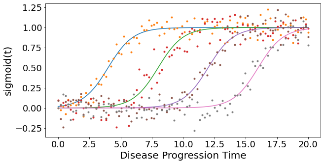
Simulate some data#
N = 4   # number of events/features
J = 100 # number of patients

noise_scale = 0.1

dp = np.linspace(0, 20, J)
def sigmoid(t,a=1,b=-10):
    return 1/(1 + np.exp(-a*(t-b)))

gradients = np.array([1,1,1,1])
onsets    = np.array([4,8,12,16])

X = np.empty(shape=(J,N))
fig,ax = plt.subplots(figsize=(10,5))
for a,b,k in zip(gradients,onsets,range(len(gradients))):
    # print('a = %i, b = %i' % (a,b))
    x = sigmoid(t=dp,a=a,b=b)
    #print(x)
    ax.plot(dp, x)
    y = x + np.random.normal(0, noise_scale, x.size)
    X[:,k] = y
    ax.plot(dp, y,'.')

ax.set_xlabel("Disease Progression Time",fontsize=20)
ax.set_ylabel("sigmoid(t)",fontsize=20)
Text(0, 0.5, 'sigmoid(t)')
#* Sample some controls
X_controls = np.empty(shape=X.shape)
for k in range(len(gradients)):
    X_controls[:,k] = np.random.normal(0, 0.05, (X_controls.shape[0],))
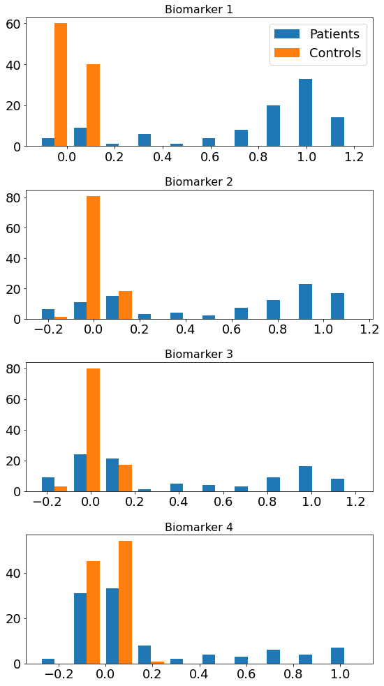
Didactic step: Look at the data#
Visual: look at the histograms of patients and controls
Statistical tests: use null hypothesis statistical tests of “differences” to select features
Loosely speaking, a significant difference suggests presence of “disease signal” (patient measurements are “different” to controls measurements) in a biomarker
#* 1. Histograms
fig,ax = plt.subplots(N,1,figsize=(8,14))
for k in range(N):
    ax[k].hist([ X[:,k],X_controls[:,k]],label=['Patients','Controls'])
    ax[k].set_title('Biomarker %i' % (k+1),fontsize=16)
ax[0].legend()
fig.tight_layout()
Basic statistical tests#
Effect size: (difference in medians) / (“width” of controls distribution)
Mann-Whitney U test (quoting Wikipedia):
a nonparametric test of the null hypothesis that, for randomly selected values X and Y from two populations, the probability of X being greater than Y is equal to the probability of Y being greater than X.
#* 2. Basic statistics
# I use a nonparametric test because it works regardless of the data distributions
# (some tests assume some level of Gaussianity)
from scipy import stats
print('Mann Whitney U test')

for k in range(N):
    x_c = X_controls[:,k]
    x_p = X[:,k]
    effect_size = np.absolute(np.median(x_p)-np.median(x_c))/stats.median_abs_deviation(x_c)
    u,p = stats.mannwhitneyu(x_c,x_p)
    print('Biomarker %i\n - effect size = %.3g\n - u = %i, p = %.2g' % (k+1,effect_size,u,p))
Mann Whitney U test
Biomarker 1
 - effect size = 26.3
 - u = 448, p = 9.9e-29
Biomarker 2
 - effect size = 26.4
 - u = 1260, p = 6.4e-20
Biomarker 3
 - effect size = 4.29
 - u = 2215, p = 1e-11
Biomarker 4
 - effect size = 1.54
 - u = 3676, p = 0.0012
Prepare data for fitting#
Data matrix X has M individuals (patients, controls, prodromal/at-risk individuals) and N biomarkers/events
#* Setup data for fitting
y          = np.ones(shape=(X.shape[0],1))
y_controls = np.zeros(shape=(X_controls.shape[0],1))

X_patients_controls = np.concatenate((X,X_controls),axis=0)
y_patients_controls = np.concatenate((y,y_controls),axis=0)

X = X_patients_controls
y = y_patients_controls.flatten().astype(int)
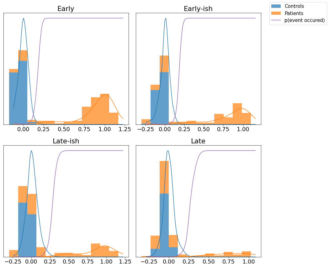
Fit mixture models#
This step maps biomarker values x (columns of data matrix X) to p(event), allowing for patients to be at different stages of cumulative abnormality.
Typical group-level analyses simply compare measurements from patients with controls, e.g., looking for statistical “differences” in the mean values. The mixture model allows for patients to have both abnormal observations that deviate from controls (these are early disease events), and normal observations (these will be later disease events)
from kde_ebm.mixture_model import fit_all_kde_models, fit_all_gmm_models, get_prob_mat

from kde_ebm.plotting import mixture_model_grid, mcmc_uncert_mat, mcmc_trace, stage_histogram

from kde_ebm.mcmc import mcmc, parallel_bootstrap, bootstrap_ebm, bootstrap_ebm_fixedMM, bootstrap_ebm_return_mixtures
#* Label the biomarkers/events
e = ['Early','Early-ish','Late-ish','Late']
e_labels = e
#* Direction of progression (1 = biomarker increases in patients; -1 = biomarker decreases in patients)
#  This is a feature of the KDE EBM software.
e_disease_direction_dict = {'Early':1,'Early-ish':1,'Late-ish':1,'Late':1}
e_disease_direction = [e_disease_direction_dict[f] for f in e]
kde_mixtures = fit_all_kde_models(
    X, y,
    implement_fixed_controls = True,
    patholog_dirn_array      = e_disease_direction
)
#* View the mixture models
mixture_model_grid(
    X,y,
    kde_mixtures,
    score_names=e,
    class_names=['Controls','Patients']
)
(<Figure size 864x864 with 4 Axes>,
 array([[<AxesSubplot:title={'center':'Early'}>,
         <AxesSubplot:title={'center':'Early-ish'}>],
        [<AxesSubplot:title={'center':'Late-ish'}>,
         <AxesSubplot:title={'center':'Late'}>]], dtype=object))
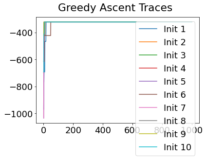
Sequencing using MCMC: Markov Chain Monte Carlo#
This is a standard method for approximating a model posterior when exact inference is intractable.
Here we are performing maximum likelihood inference. The EBM posterior is intractable in general because evaluating the likelihood function requires calculating the likelihood of all N! possible sequences for N biomarkers.
This quickly explodes for N > 6, so we generate random samples from the posterior (the full set of possible sequences) using MCMC, and keep only those sequences that increase the likelihood (ideally towards the maximum).
In general, the posterior won’t be a convex function, i.e., one having a single easy-to-find maximum.
In practice, the posterior could consist of multiple maxima at different locations in parameter space. To avoid getting “stuck” in a local maximum, we follow good machine learning practice when searching parameter space to sample from the posterior: multiple random initialisations of the sampling, greedy initialisation, and MCMC sampling.
Details of the bespoke MCMC algorithm used here are in the original EBM paper: Fonteijn et al., NeuroImage (2012).
#* MCMC sequencing
mcmc_samples = mcmc(X, kde_mixtures)
#* Maximum Likelihood sequence over all samples
seq_ml = mcmc_samples[0].ordering
# print('ML sequence: {0}'.format(seq_ml))
print('ML order   : %s' % ', '.join([e_labels[k] for k in seq_ml]))
100%|███████████████████████████████████████████████████████████████████████████████████████████████████████████████████████████████████████████████████| 1000/1000 [00:00<00:00, 9227.13it/s]
100%|███████████████████████████████████████████████████████████████████████████████████████████████████████████████████████████████████████████████████| 1000/1000 [00:00<00:00, 9427.65it/s]
100%|███████████████████████████████████████████████████████████████████████████████████████████████████████████████████████████████████████████████████| 1000/1000 [00:00<00:00, 9329.24it/s]
100%|███████████████████████████████████████████████████████████████████████████████████████████████████████████████████████████████████████████████████| 1000/1000 [00:00<00:00, 9782.61it/s]
100%|███████████████████████████████████████████████████████████████████████████████████████████████████████████████████████████████████████████████████| 1000/1000 [00:00<00:00, 9975.96it/s]
100%|██████████████████████████████████████████████████████████████████████████████████████████████████████████████████████████████████████████████████| 1000/1000 [00:00<00:00, 10124.42it/s]
100%|███████████████████████████████████████████████████████████████████████████████████████████████████████████████████████████████████████████████████| 1000/1000 [00:00<00:00, 9642.83it/s]
100%|███████████████████████████████████████████████████████████████████████████████████████████████████████████████████████████████████████████████████| 1000/1000 [00:00<00:00, 9292.14it/s]
100%|███████████████████████████████████████████████████████████████████████████████████████████████████████████████████████████████████████████████████| 1000/1000 [00:00<00:00, 9534.26it/s]
100%|███████████████████████████████████████████████████████████████████████████████████████████████████████████████████████████████████████████████████| 1000/1000 [00:00<00:00, 9663.72it/s]
/usr/local/lib/python3.9/site-packages/kde_ebm/mcmc/mcmc.py:39: UserWarning: Matplotlib is currently using module://matplotlib_inline.backend_inline, which is a non-GUI backend, so cannot show the figure.
  fig.show()
100%|█████████████████████████████████████████████████████████████████████████████████████████████████████████████████████████████████████████████████| 10000/10000 [00:01<00:00, 9444.17it/s]
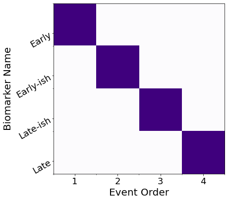
ML order : Early, Early-ish, Late-ish, Late
# View the ML posterior
f,a = mcmc_uncert_mat(mcmc_samples, ml_order=None, score_names=e_labels)
# Save in a dict()
ebm_results = {"mixtures": kde_mixtures, "mcmc_samples": mcmc_samples, "sequence_ml": seq_ml}
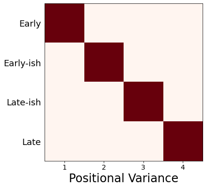
Example of how to tweak the output positional variance diagram#
I define some convenience functions, then use them to plot
import itertools
def extract_pvd(ml_order,samples):
    if type(ml_order) is list:
        #* List of PVDs from cross-validation/bootstrapping
        n_ = len(ml_order[0])
        pvd = np.zeros((n_,n_))
        #all_orders = np.array(ml_order)
        if type(samples[0]) is list:
            #* 10-fold CV returns MCMC samples for each fold separately in a list - concatenate them here
            all_samples = list(itertools.chain.from_iterable(samples))
        else:
            #* Bootstrapping returns MCMC samples pre-concatenated
            all_samples = samples
        all_orders = np.array([x.ordering for x in all_samples])
        for i in range(n_):
            pvd[i, :] = np.sum(all_orders == ml_order[0][i], axis=0)
        #pvd_cv, cv_rank = reorder_PVD_average_ranking(PVD=pvd)
        pvd, rank = reorder_PVD(pvd)
        seq = [ml_order[0][i] for i in rank]
    else:
        #* Single PVD (ML results)
        n_ = len(ml_order)
        pvd = np.zeros((n_,n_))
        samples_ = np.array([x.ordering for x in samples])
        seq = ml_order
        for i in range(n_):
            pvd[i, :] = np.sum(samples_ == seq[i], axis=0)
    return pvd, seq

def reorder_PVD(PVD,mean_bool=False,edf_threshold=0.5):
    """
    Reorders a PVD by scoring the frequencies in each row, then ranking in increasing order.

    Score: integral of complementary empirical distribution (1-EDF) up to a threshold.
    Rationale: the sooner the EDF gets to the threshold, the earlier it should be in the ranking.

    """

    if mean_bool:
        n_ = PVD.shape[0]
        ranking = np.linspace(1,n_,n_) # weights
        weights = PVD
        mean_rank = []
        for i in range(n_):
            mean_rank.append( sum( weights[i,:] * ranking ) / sum(weights[i,:]) )
        new_order = np.argsort(mean_rank)
    else:
        #* Find where the empirical distribution first exceeds the threshold
        edf = np.cumsum(PVD,axis=1)
        edf = edf / np.tile(np.max(edf,axis=1).reshape(-1,1),(1,edf.shape[1]))
        edf_above_threshold = []
        for k in range(edf.shape[0]):
            edf_above_threshold.append(np.where(edf[k,:]>=edf_threshold)[0][0])
        #* Ties implicitly split by original ordering in the PVD (likely the ML ordering)
        edf_rank = np.argsort(edf_above_threshold)
        new_order = edf_rank

    PVD_new = PVD[new_order,:]
    # PVD_new = np.zeros((n_,n_))
    # for i in range(n_):
    #     PVD_new[i, :] = PVD[new_order[i],:]

    return PVD_new, new_order

# Frontiers default is pdf with 300dpi
# And run it all through imagemagick after to convert
def save_plot(fig, fname, fig_format="png", dpi=150, **kwargs):
    fig.savefig(
        f"{fname}.{fig_format}",
        dpi=300,
        bbox_inches="tight",
        **kwargs
    )
# Get labels
nom = 'tute'
#* Plot EBM (PVD)
pvd_ml, seq_ml = extract_pvd(ml_order=seq_ml,samples=mcmc_samples)
reorder_ml = np.argsort(seq_ml)
pvd_ml_ = pvd_ml[:][reorder_ml]

fig, ax = plt.subplots(1,1,figsize=(9, 6),sharey=False)
labels = e_labels
labels_ = [labels[i].replace('TOTAL','').replace('TOT','').replace('-detrended','') for i in seq_ml]
ax.imshow(pvd_ml_[:][seq_ml], interpolation='nearest', cmap='Reds')

n_biomarkers = pvd_ml.shape[0]
stp = 1
fs = 14
tick_marks_x = np.arange(0,n_biomarkers,stp)
x_labs = range(1, n_biomarkers+1,stp)
ax.set_xticks(tick_marks_x)
ax.set_xticklabels(x_labs, rotation=0,fontsize=fs)
tick_marks_y = np.arange(n_biomarkers)
ax.set_yticks(tick_marks_y+0.0)
ax.tick_params(axis='y',color='w')
labels_trimmed = [x[2:].replace('_', ' ') if x.startswith('p_') else x.replace('_', ' ') for x in labels_]
ax.set_yticklabels(labels_trimmed,#,np.array(labels_trimmed, dtype='object')[seq_],
                   rotation=0, #ha='right',
                   rotation_mode='anchor',
                   fontsize=18)
# ax.set_ylabel('Instrument', fontsize=28)
ax.set_xlabel('Positional Variance', fontsize=24)
ax.grid(False)

save_plot(fig, nom+"-PVD_ML")
Patient staging utility#
Concept: align individuals to the model
Method (see Young et al, Brain 2014): compare data from each individual (patients/controls/at-risk) with the model and calculate a p(event) vector, then assign the most likely stage according to the accumulation of disease events
#* Define the EBM staging function
def ebm_staging(x,mixtures,samples):
    """
    Given a trained EBM (mixture_models,mcmc_samples), and correctly-formatted data, stage the data
    NOTE: To use CV-EBMs, you'll need to call this for each fold, then combine.
    Author: Neil P Oxtoby, UCL, September 2018
    """
    if type(mixtures[0]) is list:
        #* List of mixture models from cross-validation / bootstrapping
        n_cv = len(mixtures)
        prob_mat = []
        stages = []
        stage_likelihoods = []
        stages_expected = []
        for k in range(n_cv):
            #* Stage the data
            prob_mat.append(get_prob_mat(x, mixtures[k]))
            stages_k, stage_likelihoods_k = samples[k][0].stage_data(prob_mat[k])
            stages.append(stages_k)
            stage_likelihoods.append(stage_likelihoods_k)
            #* Average (expectation value) stage
            stages_expected_k = np.ndarray(shape=stages_k.shape)
            for kk in range(stages_expected_k.shape[0]):
                stages_expected_k[kk] = np.sum(stage_likelihoods_k[kk,:]*np.arange(1,stage_likelihoods_k.shape[1]+1,1))/np.sum(stage_likelihoods_k[kk,:]) - 1
            stages_expected.append(stages_expected_k)
    else:
        #* Stage the data
        prob_mat = get_prob_mat(x, mixtures)
        if type(samples[0]) is list:
            n_bs = len(samples)
            stages = []
            stage_likelihoods = []
            stages_expected = []
            for k in range(n_bs):
                #* Stage the data
                stages_k, stage_likelihoods_k = samples[k][0].stage_data(prob_mat)
                stages.append(stages_k)
                stage_likelihoods.append(stage_likelihoods_k)
                #* Average (expectation value) stage
                stages_expected_k = np.ndarray(shape=stages_k.shape)
                for kk in range(stages_expected_k.shape[0]):
                    stages_expected_k[kk] = np.sum(stage_likelihoods_k[kk,:]*np.arange(1,stage_likelihoods_k.shape[1]+1,1))/np.sum(stage_likelihoods_k[kk,:]) - 1
                stages_expected.append(stages_expected_k)
        else:
            stages, stage_likelihoods = samples[0].stage_data(prob_mat)
            #* Average (expectation value) stage
            stages_expected = np.ndarray(shape=stages.shape)
            for k in range(stages_expected.shape[0]):
                stages_expected[k] = np.sum(stage_likelihoods[k,:]*np.arange(1,stage_likelihoods.shape[1]+1,1))/np.sum(stage_likelihoods[k,:]) - 1
    # #* Average (expectation value) stage
    # stages_expected_n = np.sum(stage_likelihoods,axis=1)
    # stages_expected_ = np.average(stage_likelihoods_long_ml,axis=1,weights=np.arange(1,stage_likelihoods_long_ml.shape[1]+1,1))
    # stages_expected_ = stages_expected_/stages_expected_n

    return prob_mat, stages, stage_likelihoods, stages_expected
#* Staging
#* Maximum-likelihood model stage: could include longitudinal data, including followups not used to train the EBM
prob_mat_ml, stages_long_ml, stage_likelihoods_long_ml, stages_long_ml_expected = ebm_staging(
    x=X,
    mixtures=kde_mixtures,
    samples=mcmc_samples
)
stages_long = stages_long_ml
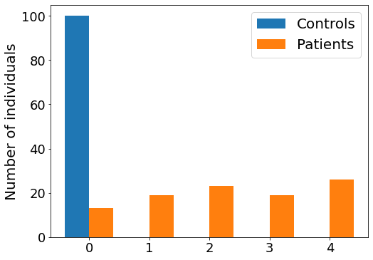
Plot a staging histogram#
Number of individuals in each EBM stage
fig, ax = plt.subplots(figsize=(8,6))

ax.hist([ stages_long[y==0], stages_long[y==1]],bins=np.arange(-0.5,N+1.5,1))
# #* Seaborn version: requires creating a Pandas DataFrame and adding data/etc.
# ax = sns.histplot(
#     data = df_staging,
#     x    = stage_column,
#     hue  = "Status",
#     ax   = ax
#     discrete  = True,
#     multiple  = "dodge",
#     log_scale = (False, True),
#     palette   = status_palette,
# )
ax.set_ylabel('Number of individuals',fontsize=20)
ax.legend(['Controls','Patients'],fontsize=20)
<matplotlib.legend.Legend at 0x127811790>
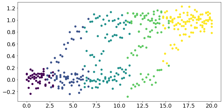
#* Plot the original data, coloured by stage
fig,ax = plt.subplots(figsize=(12,6))

for k in range(N):
    plt.scatter(dp,X[y==1,k],c=stages_long[y==1],cmap='viridis',label='')
plt.plot
# ax.legend(['Stage %i' % k for k in range(N)],loc='center right',bbox_to_anchor=[1.5,0.5])
<function matplotlib.pyplot.plot(*args, scalex=True, scaley=True, data=None, **kwargs)>
Bonus: Cross-validation#
Generalizability/robustness of a model can be quantified by testing the model on independent data, i.e., data not included when training the model.
Cross-validation does this by splitting the available data into train/test sets.
k-fold cross-validation#
Splitting a dataset into k “folds” enables calculation of model performance statistics (e.g., mean, standard deviation) over k test sets, using the other k-1 folds to train the model each time.
It is common to use k=10, which amounts to using 90% of your data to train and 10% to test.
This process can be repeated multiple times using different random partitions (splits) into folds.

By Gufosowa - Own work, CC BY-SA 4.0, https://commons.wikimedia.org/w/index.php?curid=82298768
from sklearn.model_selection import RepeatedStratifiedKFold

# More convenience functions: YMMV
def ebm_2_run(x,y,events,
              kde_flag=True,
              verbose_flag = False,
              plot_flag = False,
              export_plot_flag = True,
              implement_fixed_controls=True,
              patholog_dirn_array=None
              ):
    """
    Build a KDE EBM from the data in df_EBM[events]
    Author: Neil P. Oxtoby, UCL, September 2018
    """
    #* Fit the mixture models
    if kde_flag:
        mixtures = fit_all_kde_models(x, y, implement_fixed_controls=implement_fixed_controls, patholog_dirn_array=patholog_dirn_array)
    else:
        mixtures = fit_all_gmm_models(x, y, implement_fixed_controls=implement_fixed_controls)
    #* MCMC sequencing
    mcmc_samples = mcmc(x, mixtures)
    ml_order = mcmc_samples[0].ordering # max-like order
    #* Print out the biomarkers in ML order
    if verbose_flag:
        for k in range(len(ml_order)):
            print('ML order: {0}'.format(events[ml_order[k]]))
    if plot_flag:
        #* Plot the positional variance diagram
        events_labels = [l.replace('-detrended','') for l in events]
        fig, ax = mcmc_uncert_mat(mcmc_samples, score_names=events_labels)
        fig.tight_layout()
        ax.tick_params(axis='both', which='major', labelsize=14)
        ax.yaxis.label.set_size(24)
        ax.xaxis.label.set_size(24)
        fig.set_figwidth(14)
        fig.set_figheight(14)
        #* Export figure
        if export_plot_flag:
            f_name = 'PPMI-EBM-PVD.png' # FIXME: add timestamp
            fig.savefig(f_name,dpi=300)

    return mixtures, mcmc_samples, ml_order

def ebm_3_staging(x,mixtures,samples):
    """
    Given a trained EBM (mixture_models,mcmc_samples), and correctly-formatted data, stage the data
    NOTE: To use CV-EBMs, you'll need to call this for each fold, then combine.
    Author: Neil P Oxtoby, UCL, September 2018
    """
    if type(mixtures[0]) is list:
        #* List of mixture models from cross-validation / bootstrapping
        n_cv = len(mixtures)
        prob_mat = []
        stages = []
        stage_likelihoods = []
        stages_expected = []
        for k in range(n_cv):
            #* Stage the data
            prob_mat.append(get_prob_mat(x, mixtures[k]))
            stages_k, stage_likelihoods_k = samples[k][0].stage_data(prob_mat[k])
            stages.append(stages_k)
            stage_likelihoods.append(stage_likelihoods_k)
            #* Average (expectation value) stage
            stages_expected_k = np.ndarray(shape=stages_k.shape)
            for kk in range(stages_expected_k.shape[0]):
                stages_expected_k[kk] = np.sum(stage_likelihoods_k[kk,:]*np.arange(1,stage_likelihoods_k.shape[1]+1,1))/np.sum(stage_likelihoods_k[kk,:]) - 1
            stages_expected.append(stages_expected_k)
    else:
        #* Stage the data
        prob_mat = get_prob_mat(x, mixtures)
        if type(samples[0]) is list:
            n_bs = len(samples)
            stages = []
            stage_likelihoods = []
            stages_expected = []
            for k in range(n_bs):
                #* Stage the data
                stages_k, stage_likelihoods_k = samples[k][0].stage_data(prob_mat)
                stages.append(stages_k)
                stage_likelihoods.append(stage_likelihoods_k)
                #* Average (expectation value) stage
                stages_expected_k = np.ndarray(shape=stages_k.shape)
                for kk in range(stages_expected_k.shape[0]):
                    stages_expected_k[kk] = np.sum(stage_likelihoods_k[kk,:]*np.arange(1,stage_likelihoods_k.shape[1]+1,1))/np.sum(stage_likelihoods_k[kk,:]) - 1
                stages_expected.append(stages_expected_k)
        else:
            stages, stage_likelihoods = samples[0].stage_data(prob_mat)
            #* Average (expectation value) stage
            stages_expected = np.ndarray(shape=stages.shape)
            for k in range(stages_expected.shape[0]):
                stages_expected[k] = np.sum(stage_likelihoods[k,:]*np.arange(1,stage_likelihoods.shape[1]+1,1))/np.sum(stage_likelihoods[k,:]) - 1
    # #* Average (expectation value) stage
    # stages_expected_n = np.sum(stage_likelihoods,axis=1)
    # stages_expected_ = np.average(stage_likelihoods_long_ml,axis=1,weights=np.arange(1,stage_likelihoods_long_ml.shape[1]+1,1))
    # stages_expected_ = stages_expected_/stages_expected_n

    return prob_mat, stages, stage_likelihoods, stages_expected

def ebm_2_repeatedcv(x,y,events,
             rcv_folds=RepeatedStratifiedKFold(n_splits=5, n_repeats=5, random_state=None),
             kde_flag=True,
             plot_each_fold=False,
             implement_fixed_controls=True,
             patholog_dirn_array=None,
             model_stage=None
             ):
    """
    Run repeated k-fold cross-validation
        Uses ML model stage for CV accuracy: stage test set for each training set
    Author: Neil P Oxtoby, UCL, November 2019
    """
    mixtures_cv = []
    mcmc_samples_cv = []
    ml_orders_cv = []
    staging_errors_cv = []
    test_set_size_cv = []

    f = 0
    for train_index, test_index in rcv_folds.split(x, y):
        x_train, x_test = x[train_index], x[test_index]
        y_train, y_test = y[train_index], y[test_index]
        stages_test_groundtruth = model_stage[test_index]
        #* Fit
        mixtures_k, mcmc_samples_k, ml_order_k = ebm_2_run(
            x_train,y_train,
            events,
            kde_flag=kde_flag,
            plot_flag=plot_each_fold,
            implement_fixed_controls=implement_fixed_controls,
            patholog_dirn_array=patholog_dirn_array
        )
        #* Save
        mixtures_cv.append(mixtures_k)
        mcmc_samples_cv.append(mcmc_samples_k)
        ml_orders_cv.append(ml_order_k)
        #* Stage
        prob_mat_test, stages_test, stage_likelihoods_test, stages_long_test = ebm_3_staging(x=x_test, mixtures=mixtures_k, samples=mcmc_samples_k)
        staging_errors_cv.append([stages_test-stages_test_groundtruth])
        f+=1
        print('Repeated CV fold {0} of {1}'.format(f,rcv_folds.get_n_splits()))
    return mixtures_cv, mcmc_samples_cv, ml_orders_cv, staging_errors_cv
#* RCV1: Repeated, stratified 5-fold CV - uses ML stage as ground truth for test folds
k_folds = 5
n_repeats = 10

repeated_cvfolds = RepeatedStratifiedKFold(n_splits=k_folds, n_repeats=n_repeats) #, random_state=36851234)
if 'ebm_results' in locals():
    check = True
else:
    check = False


if check:
    if "mixtures_rcv" in ebm_results:
        kde_mixtures_rcv = ebm_results["mixtures_rcv"]
        mcmc_samples_rcv = ebm_results["mcmc_samples_rcv"]
        seqs_rcv = ebm_results["sequences_rcv"]
        staging_errors_rcv = ebm_results["staging_errors_rcv"]
        runit = False
    else:
        runit = True
else:
    runit = True

if runit:
    kde_mixtures_rcv, mcmc_samples_rcv, seqs_rcv, staging_errors_rcv = ebm_2_repeatedcv(
        x=X,
        y=y,
        events=e,
        rcv_folds=repeated_cvfolds,
        implement_fixed_controls=True,
        patholog_dirn_array=e_disease_direction,
        model_stage=stages_long
    )
    #* Save
    ebm_results["mixtures_rcv"] = kde_mixtures_rcv
    ebm_results["mcmc_samples_rcv"] = mcmc_samples_rcv
    ebm_results["sequences_rcv"] = seqs_rcv
    ebm_results["staging_errors_rcv"] = staging_errors_rcv
    # pickle_file = open(pickle_path,'wb')
    # pickle_output = pickle.dump(ebm_results, pickle_file)
    # pickle_file.close()
100%|██████████████████████████████████████████████████████████████████████████████████████████████████████████████████████████████████████████████████| 1000/1000 [00:00<00:00, 10426.54it/s]
100%|██████████████████████████████████████████████████████████████████████████████████████████████████████████████████████████████████████████████████| 1000/1000 [00:00<00:00, 10409.17it/s]
100%|██████████████████████████████████████████████████████████████████████████████████████████████████████████████████████████████████████████████████| 1000/1000 [00:00<00:00, 10132.03it/s]
100%|██████████████████████████████████████████████████████████████████████████████████████████████████████████████████████████████████████████████████| 1000/1000 [00:00<00:00, 10279.17it/s]
100%|██████████████████████████████████████████████████████████████████████████████████████████████████████████████████████████████████████████████████| 1000/1000 [00:00<00:00, 10308.18it/s]
100%|██████████████████████████████████████████████████████████████████████████████████████████████████████████████████████████████████████████████████| 1000/1000 [00:00<00:00, 10454.55it/s]
100%|██████████████████████████████████████████████████████████████████████████████████████████████████████████████████████████████████████████████████| 1000/1000 [00:00<00:00, 10370.13it/s]
100%|██████████████████████████████████████████████████████████████████████████████████████████████████████████████████████████████████████████████████| 1000/1000 [00:00<00:00, 10325.76it/s]
100%|███████████████████████████████████████████████████████████████████████████████████████████████████████████████████████████████████████████████████| 1000/1000 [00:00<00:00, 9999.60it/s]
100%|██████████████████████████████████████████████████████████████████████████████████████████████████████████████████████████████████████████████████| 1000/1000 [00:00<00:00, 10294.74it/s]
/usr/local/lib/python3.9/site-packages/kde_ebm/mcmc/mcmc.py:39: UserWarning: Matplotlib is currently using module://matplotlib_inline.backend_inline, which is a non-GUI backend, so cannot show the figure.
  fig.show()
100%|█████████████████████████████████████████████████████████████████████████████████████████████████████████████████████████████████████████████████| 10000/10000 [00:01<00:00, 9456.70it/s]
100%|██████████████████████████████████████████████████████████████████████████████████████████████████████████████████████████████████████████████████| 1000/1000 [00:00<00:00, 10282.88it/s]
  0%|                                                                                                                                                                | 0/1000 [00:00<?, ?it/s]
Repeated CV fold 1 of 50
100%|███████████████████████████████████████████████████████████████████████████████████████████████████████████████████████████████████████████████████| 1000/1000 [00:00<00:00, 9386.84it/s]
100%|██████████████████████████████████████████████████████████████████████████████████████████████████████████████████████████████████████████████████| 1000/1000 [00:00<00:00, 10362.81it/s]
100%|███████████████████████████████████████████████████████████████████████████████████████████████████████████████████████████████████████████████████| 1000/1000 [00:00<00:00, 9826.59it/s]
100%|██████████████████████████████████████████████████████████████████████████████████████████████████████████████████████████████████████████████████| 1000/1000 [00:00<00:00, 10408.76it/s]
100%|██████████████████████████████████████████████████████████████████████████████████████████████████████████████████████████████████████████████████| 1000/1000 [00:00<00:00, 10513.41it/s]
100%|███████████████████████████████████████████████████████████████████████████████████████████████████████████████████████████████████████████████████| 1000/1000 [00:00<00:00, 9445.99it/s]
100%|██████████████████████████████████████████████████████████████████████████████████████████████████████████████████████████████████████████████████| 1000/1000 [00:00<00:00, 10265.59it/s]
100%|██████████████████████████████████████████████████████████████████████████████████████████████████████████████████████████████████████████████████| 1000/1000 [00:00<00:00, 10102.33it/s]
100%|██████████████████████████████████████████████████████████████████████████████████████████████████████████████████████████████████████████████████| 1000/1000 [00:00<00:00, 10322.15it/s]
/usr/local/lib/python3.9/site-packages/kde_ebm/mcmc/mcmc.py:39: UserWarning: Matplotlib is currently using module://matplotlib_inline.backend_inline, which is a non-GUI backend, so cannot show the figure.
  fig.show()
100%|█████████████████████████████████████████████████████████████████████████████████████████████████████████████████████████████████████████████████| 10000/10000 [00:01<00:00, 9799.52it/s]
100%|███████████████████████████████████████████████████████████████████████████████████████████████████████████████████████████████████████████████████| 1000/1000 [00:00<00:00, 9566.08it/s]
  0%|                                                                                                                                                                | 0/1000 [00:00<?, ?it/s]
Repeated CV fold 2 of 50
100%|███████████████████████████████████████████████████████████████████████████████████████████████████████████████████████████████████████████████████| 1000/1000 [00:00<00:00, 9989.32it/s]
100%|██████████████████████████████████████████████████████████████████████████████████████████████████████████████████████████████████████████████████| 1000/1000 [00:00<00:00, 10381.74it/s]
100%|██████████████████████████████████████████████████████████████████████████████████████████████████████████████████████████████████████████████████| 1000/1000 [00:00<00:00, 10619.43it/s]
100%|██████████████████████████████████████████████████████████████████████████████████████████████████████████████████████████████████████████████████| 1000/1000 [00:00<00:00, 10539.86it/s]
100%|██████████████████████████████████████████████████████████████████████████████████████████████████████████████████████████████████████████████████| 1000/1000 [00:00<00:00, 10020.03it/s]
100%|██████████████████████████████████████████████████████████████████████████████████████████████████████████████████████████████████████████████████| 1000/1000 [00:00<00:00, 10569.50it/s]
100%|██████████████████████████████████████████████████████████████████████████████████████████████████████████████████████████████████████████████████| 1000/1000 [00:00<00:00, 10235.95it/s]
100%|███████████████████████████████████████████████████████████████████████████████████████████████████████████████████████████████████████████████████| 1000/1000 [00:00<00:00, 9391.28it/s]
100%|██████████████████████████████████████████████████████████████████████████████████████████████████████████████████████████████████████████████████| 1000/1000 [00:00<00:00, 10364.85it/s]
/usr/local/lib/python3.9/site-packages/kde_ebm/mcmc/mcmc.py:39: UserWarning: Matplotlib is currently using module://matplotlib_inline.backend_inline, which is a non-GUI backend, so cannot show the figure.
  fig.show()
100%|█████████████████████████████████████████████████████████████████████████████████████████████████████████████████████████████████████████████████| 10000/10000 [00:01<00:00, 9761.18it/s]
100%|██████████████████████████████████████████████████████████████████████████████████████████████████████████████████████████████████████████████████| 1000/1000 [00:00<00:00, 10172.65it/s]
  0%|                                                                                                                                                                | 0/1000 [00:00<?, ?it/s]
Repeated CV fold 3 of 50
100%|███████████████████████████████████████████████████████████████████████████████████████████████████████████████████████████████████████████████████| 1000/1000 [00:00<00:00, 9760.76it/s]
100%|██████████████████████████████████████████████████████████████████████████████████████████████████████████████████████████████████████████████████| 1000/1000 [00:00<00:00, 10120.44it/s]
100%|██████████████████████████████████████████████████████████████████████████████████████████████████████████████████████████████████████████████████| 1000/1000 [00:00<00:00, 10181.44it/s]
100%|███████████████████████████████████████████████████████████████████████████████████████████████████████████████████████████████████████████████████| 1000/1000 [00:00<00:00, 9388.00it/s]
100%|███████████████████████████████████████████████████████████████████████████████████████████████████████████████████████████████████████████████████| 1000/1000 [00:00<00:00, 9691.11it/s]
100%|███████████████████████████████████████████████████████████████████████████████████████████████████████████████████████████████████████████████████| 1000/1000 [00:00<00:00, 9616.21it/s]
100%|███████████████████████████████████████████████████████████████████████████████████████████████████████████████████████████████████████████████████| 1000/1000 [00:00<00:00, 9996.98it/s]
100%|███████████████████████████████████████████████████████████████████████████████████████████████████████████████████████████████████████████████████| 1000/1000 [00:00<00:00, 9889.03it/s]
100%|███████████████████████████████████████████████████████████████████████████████████████████████████████████████████████████████████████████████████| 1000/1000 [00:00<00:00, 9677.52it/s]
/usr/local/lib/python3.9/site-packages/kde_ebm/mcmc/mcmc.py:39: UserWarning: Matplotlib is currently using module://matplotlib_inline.backend_inline, which is a non-GUI backend, so cannot show the figure.
  fig.show()
100%|█████████████████████████████████████████████████████████████████████████████████████████████████████████████████████████████████████████████████| 10000/10000 [00:01<00:00, 9482.59it/s]
100%|██████████████████████████████████████████████████████████████████████████████████████████████████████████████████████████████████████████████████| 1000/1000 [00:00<00:00, 10247.58it/s]
  0%|                                                                                                                                                                | 0/1000 [00:00<?, ?it/s]
Repeated CV fold 4 of 50
100%|███████████████████████████████████████████████████████████████████████████████████████████████████████████████████████████████████████████████████| 1000/1000 [00:00<00:00, 9786.26it/s]
100%|██████████████████████████████████████████████████████████████████████████████████████████████████████████████████████████████████████████████████| 1000/1000 [00:00<00:00, 10040.87it/s]
100%|██████████████████████████████████████████████████████████████████████████████████████████████████████████████████████████████████████████████████| 1000/1000 [00:00<00:00, 10342.44it/s]
100%|███████████████████████████████████████████████████████████████████████████████████████████████████████████████████████████████████████████████████| 1000/1000 [00:00<00:00, 9359.53it/s]
100%|███████████████████████████████████████████████████████████████████████████████████████████████████████████████████████████████████████████████████| 1000/1000 [00:00<00:00, 9531.06it/s]
100%|███████████████████████████████████████████████████████████████████████████████████████████████████████████████████████████████████████████████████| 1000/1000 [00:00<00:00, 8922.82it/s]
100%|███████████████████████████████████████████████████████████████████████████████████████████████████████████████████████████████████████████████████| 1000/1000 [00:00<00:00, 9556.57it/s]
100%|██████████████████████████████████████████████████████████████████████████████████████████████████████████████████████████████████████████████████| 1000/1000 [00:00<00:00, 10448.80it/s]
100%|██████████████████████████████████████████████████████████████████████████████████████████████████████████████████████████████████████████████████| 1000/1000 [00:00<00:00, 10487.60it/s]
/usr/local/lib/python3.9/site-packages/kde_ebm/mcmc/mcmc.py:39: UserWarning: Matplotlib is currently using module://matplotlib_inline.backend_inline, which is a non-GUI backend, so cannot show the figure.
  fig.show()
100%|█████████████████████████████████████████████████████████████████████████████████████████████████████████████████████████████████████████████████| 10000/10000 [00:01<00:00, 9828.04it/s]
100%|███████████████████████████████████████████████████████████████████████████████████████████████████████████████████████████████████████████████████| 1000/1000 [00:00<00:00, 9980.66it/s]
  0%|                                                                                                                                                                | 0/1000 [00:00<?, ?it/s]
Repeated CV fold 5 of 50
100%|███████████████████████████████████████████████████████████████████████████████████████████████████████████████████████████████████████████████████| 1000/1000 [00:00<00:00, 9805.37it/s]
100%|██████████████████████████████████████████████████████████████████████████████████████████████████████████████████████████████████████████████████| 1000/1000 [00:00<00:00, 10028.08it/s]
100%|██████████████████████████████████████████████████████████████████████████████████████████████████████████████████████████████████████████████████| 1000/1000 [00:00<00:00, 10352.73it/s]
100%|██████████████████████████████████████████████████████████████████████████████████████████████████████████████████████████████████████████████████| 1000/1000 [00:00<00:00, 10361.53it/s]
100%|██████████████████████████████████████████████████████████████████████████████████████████████████████████████████████████████████████████████████| 1000/1000 [00:00<00:00, 10162.00it/s]
100%|██████████████████████████████████████████████████████████████████████████████████████████████████████████████████████████████████████████████████| 1000/1000 [00:00<00:00, 10005.52it/s]
100%|███████████████████████████████████████████████████████████████████████████████████████████████████████████████████████████████████████████████████| 1000/1000 [00:00<00:00, 8994.73it/s]
100%|██████████████████████████████████████████████████████████████████████████████████████████████████████████████████████████████████████████████████| 1000/1000 [00:00<00:00, 10190.04it/s]
100%|██████████████████████████████████████████████████████████████████████████████████████████████████████████████████████████████████████████████████| 1000/1000 [00:00<00:00, 10363.55it/s]
/usr/local/lib/python3.9/site-packages/kde_ebm/mcmc/mcmc.py:39: UserWarning: Matplotlib is currently using module://matplotlib_inline.backend_inline, which is a non-GUI backend, so cannot show the figure.
  fig.show()
100%|█████████████████████████████████████████████████████████████████████████████████████████████████████████████████████████████████████████████████| 10000/10000 [00:01<00:00, 9512.29it/s]
100%|██████████████████████████████████████████████████████████████████████████████████████████████████████████████████████████████████████████████████| 1000/1000 [00:00<00:00, 10361.73it/s]
  0%|                                                                                                                                                                | 0/1000 [00:00<?, ?it/s]
Repeated CV fold 6 of 50
100%|██████████████████████████████████████████████████████████████████████████████████████████████████████████████████████████████████████████████████| 1000/1000 [00:00<00:00, 10276.53it/s]
100%|██████████████████████████████████████████████████████████████████████████████████████████████████████████████████████████████████████████████████| 1000/1000 [00:00<00:00, 10315.22it/s]
100%|███████████████████████████████████████████████████████████████████████████████████████████████████████████████████████████████████████████████████| 1000/1000 [00:00<00:00, 9524.43it/s]
100%|███████████████████████████████████████████████████████████████████████████████████████████████████████████████████████████████████████████████████| 1000/1000 [00:00<00:00, 9997.51it/s]
100%|██████████████████████████████████████████████████████████████████████████████████████████████████████████████████████████████████████████████████| 1000/1000 [00:00<00:00, 10157.74it/s]
100%|███████████████████████████████████████████████████████████████████████████████████████████████████████████████████████████████████████████████████| 1000/1000 [00:00<00:00, 9520.20it/s]
100%|██████████████████████████████████████████████████████████████████████████████████████████████████████████████████████████████████████████████████| 1000/1000 [00:00<00:00, 10472.51it/s]
100%|███████████████████████████████████████████████████████████████████████████████████████████████████████████████████████████████████████████████████| 1000/1000 [00:00<00:00, 9604.48it/s]
100%|███████████████████████████████████████████████████████████████████████████████████████████████████████████████████████████████████████████████████| 1000/1000 [00:00<00:00, 9317.05it/s]
/usr/local/lib/python3.9/site-packages/kde_ebm/mcmc/mcmc.py:39: UserWarning: Matplotlib is currently using module://matplotlib_inline.backend_inline, which is a non-GUI backend, so cannot show the figure.
  fig.show()
100%|█████████████████████████████████████████████████████████████████████████████████████████████████████████████████████████████████████████████████| 10000/10000 [00:01<00:00, 9569.85it/s]
100%|██████████████████████████████████████████████████████████████████████████████████████████████████████████████████████████████████████████████████| 1000/1000 [00:00<00:00, 10221.28it/s]
  0%|                                                                                                                                                                | 0/1000 [00:00<?, ?it/s]
Repeated CV fold 7 of 50
100%|██████████████████████████████████████████████████████████████████████████████████████████████████████████████████████████████████████████████████| 1000/1000 [00:00<00:00, 10088.06it/s]
100%|██████████████████████████████████████████████████████████████████████████████████████████████████████████████████████████████████████████████████| 1000/1000 [00:00<00:00, 10331.21it/s]
100%|███████████████████████████████████████████████████████████████████████████████████████████████████████████████████████████████████████████████████| 1000/1000 [00:00<00:00, 9159.61it/s]
100%|██████████████████████████████████████████████████████████████████████████████████████████████████████████████████████████████████████████████████| 1000/1000 [00:00<00:00, 10000.01it/s]
100%|██████████████████████████████████████████████████████████████████████████████████████████████████████████████████████████████████████████████████| 1000/1000 [00:00<00:00, 10278.22it/s]
100%|██████████████████████████████████████████████████████████████████████████████████████████████████████████████████████████████████████████████████| 1000/1000 [00:00<00:00, 10230.61it/s]
100%|██████████████████████████████████████████████████████████████████████████████████████████████████████████████████████████████████████████████████| 1000/1000 [00:00<00:00, 10355.85it/s]
100%|██████████████████████████████████████████████████████████████████████████████████████████████████████████████████████████████████████████████████| 1000/1000 [00:00<00:00, 10297.39it/s]
100%|██████████████████████████████████████████████████████████████████████████████████████████████████████████████████████████████████████████████████| 1000/1000 [00:00<00:00, 10348.13it/s]
/usr/local/lib/python3.9/site-packages/kde_ebm/mcmc/mcmc.py:39: UserWarning: Matplotlib is currently using module://matplotlib_inline.backend_inline, which is a non-GUI backend, so cannot show the figure.
  fig.show()
100%|█████████████████████████████████████████████████████████████████████████████████████████████████████████████████████████████████████████████████| 10000/10000 [00:01<00:00, 9513.02it/s]
100%|███████████████████████████████████████████████████████████████████████████████████████████████████████████████████████████████████████████████████| 1000/1000 [00:00<00:00, 9148.38it/s]
  0%|                                                                                                                                                                | 0/1000 [00:00<?, ?it/s]
Repeated CV fold 8 of 50
100%|███████████████████████████████████████████████████████████████████████████████████████████████████████████████████████████████████████████████████| 1000/1000 [00:00<00:00, 8592.75it/s]
100%|███████████████████████████████████████████████████████████████████████████████████████████████████████████████████████████████████████████████████| 1000/1000 [00:00<00:00, 8632.58it/s]
100%|███████████████████████████████████████████████████████████████████████████████████████████████████████████████████████████████████████████████████| 1000/1000 [00:00<00:00, 8643.56it/s]
100%|███████████████████████████████████████████████████████████████████████████████████████████████████████████████████████████████████████████████████| 1000/1000 [00:00<00:00, 8468.71it/s]
100%|███████████████████████████████████████████████████████████████████████████████████████████████████████████████████████████████████████████████████| 1000/1000 [00:00<00:00, 8287.47it/s]
100%|███████████████████████████████████████████████████████████████████████████████████████████████████████████████████████████████████████████████████| 1000/1000 [00:00<00:00, 8654.65it/s]
100%|███████████████████████████████████████████████████████████████████████████████████████████████████████████████████████████████████████████████████| 1000/1000 [00:00<00:00, 8954.78it/s]
100%|██████████████████████████████████████████████████████████████████████████████████████████████████████████████████████████████████████████████████| 1000/1000 [00:00<00:00, 10046.84it/s]
100%|███████████████████████████████████████████████████████████████████████████████████████████████████████████████████████████████████████████████████| 1000/1000 [00:00<00:00, 9810.27it/s]
/usr/local/lib/python3.9/site-packages/kde_ebm/mcmc/mcmc.py:39: UserWarning: Matplotlib is currently using module://matplotlib_inline.backend_inline, which is a non-GUI backend, so cannot show the figure.
  fig.show()
100%|█████████████████████████████████████████████████████████████████████████████████████████████████████████████████████████████████████████████████| 10000/10000 [00:01<00:00, 8644.38it/s]
100%|██████████████████████████████████████████████████████████████████████████████████████████████████████████████████████████████████████████████████| 1000/1000 [00:00<00:00, 10206.06it/s]
  0%|                                                                                                                                                                | 0/1000 [00:00<?, ?it/s]
Repeated CV fold 9 of 50
100%|███████████████████████████████████████████████████████████████████████████████████████████████████████████████████████████████████████████████████| 1000/1000 [00:00<00:00, 9226.77it/s]
100%|███████████████████████████████████████████████████████████████████████████████████████████████████████████████████████████████████████████████████| 1000/1000 [00:00<00:00, 9053.13it/s]
100%|███████████████████████████████████████████████████████████████████████████████████████████████████████████████████████████████████████████████████| 1000/1000 [00:00<00:00, 8644.31it/s]
100%|███████████████████████████████████████████████████████████████████████████████████████████████████████████████████████████████████████████████████| 1000/1000 [00:00<00:00, 9004.23it/s]
100%|███████████████████████████████████████████████████████████████████████████████████████████████████████████████████████████████████████████████████| 1000/1000 [00:00<00:00, 8639.48it/s]
100%|███████████████████████████████████████████████████████████████████████████████████████████████████████████████████████████████████████████████████| 1000/1000 [00:00<00:00, 9375.85it/s]
100%|███████████████████████████████████████████████████████████████████████████████████████████████████████████████████████████████████████████████████| 1000/1000 [00:00<00:00, 9816.45it/s]
100%|███████████████████████████████████████████████████████████████████████████████████████████████████████████████████████████████████████████████████| 1000/1000 [00:00<00:00, 9463.15it/s]
100%|██████████████████████████████████████████████████████████████████████████████████████████████████████████████████████████████████████████████████| 1000/1000 [00:00<00:00, 10210.21it/s]
/usr/local/lib/python3.9/site-packages/kde_ebm/mcmc/mcmc.py:39: UserWarning: Matplotlib is currently using module://matplotlib_inline.backend_inline, which is a non-GUI backend, so cannot show the figure.
  fig.show()
100%|█████████████████████████████████████████████████████████████████████████████████████████████████████████████████████████████████████████████████| 10000/10000 [00:01<00:00, 9232.09it/s]
100%|███████████████████████████████████████████████████████████████████████████████████████████████████████████████████████████████████████████████████| 1000/1000 [00:00<00:00, 9409.65it/s]
  0%|                                                                                                                                                                | 0/1000 [00:00<?, ?it/s]
Repeated CV fold 10 of 50
100%|███████████████████████████████████████████████████████████████████████████████████████████████████████████████████████████████████████████████████| 1000/1000 [00:00<00:00, 8926.58it/s]
100%|███████████████████████████████████████████████████████████████████████████████████████████████████████████████████████████████████████████████████| 1000/1000 [00:00<00:00, 9606.81it/s]
100%|███████████████████████████████████████████████████████████████████████████████████████████████████████████████████████████████████████████████████| 1000/1000 [00:00<00:00, 9004.30it/s]
100%|███████████████████████████████████████████████████████████████████████████████████████████████████████████████████████████████████████████████████| 1000/1000 [00:00<00:00, 9355.69it/s]
100%|███████████████████████████████████████████████████████████████████████████████████████████████████████████████████████████████████████████████████| 1000/1000 [00:00<00:00, 8702.69it/s]
100%|███████████████████████████████████████████████████████████████████████████████████████████████████████████████████████████████████████████████████| 1000/1000 [00:00<00:00, 8891.40it/s]
100%|███████████████████████████████████████████████████████████████████████████████████████████████████████████████████████████████████████████████████| 1000/1000 [00:00<00:00, 8992.55it/s]
100%|███████████████████████████████████████████████████████████████████████████████████████████████████████████████████████████████████████████████████| 1000/1000 [00:00<00:00, 9317.22it/s]
100%|███████████████████████████████████████████████████████████████████████████████████████████████████████████████████████████████████████████████████| 1000/1000 [00:00<00:00, 9119.78it/s]
/usr/local/lib/python3.9/site-packages/kde_ebm/mcmc/mcmc.py:39: UserWarning: Matplotlib is currently using module://matplotlib_inline.backend_inline, which is a non-GUI backend, so cannot show the figure.
  fig.show()
100%|█████████████████████████████████████████████████████████████████████████████████████████████████████████████████████████████████████████████████| 10000/10000 [00:01<00:00, 8776.49it/s]
100%|███████████████████████████████████████████████████████████████████████████████████████████████████████████████████████████████████████████████████| 1000/1000 [00:00<00:00, 8638.20it/s]
  0%|                                                                                                                                                                | 0/1000 [00:00<?, ?it/s]
Repeated CV fold 11 of 50
100%|███████████████████████████████████████████████████████████████████████████████████████████████████████████████████████████████████████████████████| 1000/1000 [00:00<00:00, 8932.58it/s]
100%|███████████████████████████████████████████████████████████████████████████████████████████████████████████████████████████████████████████████████| 1000/1000 [00:00<00:00, 9548.35it/s]
100%|███████████████████████████████████████████████████████████████████████████████████████████████████████████████████████████████████████████████████| 1000/1000 [00:00<00:00, 9356.23it/s]
100%|███████████████████████████████████████████████████████████████████████████████████████████████████████████████████████████████████████████████████| 1000/1000 [00:00<00:00, 8502.23it/s]
100%|███████████████████████████████████████████████████████████████████████████████████████████████████████████████████████████████████████████████████| 1000/1000 [00:00<00:00, 8989.33it/s]
100%|███████████████████████████████████████████████████████████████████████████████████████████████████████████████████████████████████████████████████| 1000/1000 [00:00<00:00, 8806.48it/s]
100%|███████████████████████████████████████████████████████████████████████████████████████████████████████████████████████████████████████████████████| 1000/1000 [00:00<00:00, 8827.46it/s]
100%|███████████████████████████████████████████████████████████████████████████████████████████████████████████████████████████████████████████████████| 1000/1000 [00:00<00:00, 8523.40it/s]
100%|███████████████████████████████████████████████████████████████████████████████████████████████████████████████████████████████████████████████████| 1000/1000 [00:00<00:00, 8564.65it/s]
/usr/local/lib/python3.9/site-packages/kde_ebm/mcmc/mcmc.py:39: UserWarning: Matplotlib is currently using module://matplotlib_inline.backend_inline, which is a non-GUI backend, so cannot show the figure.
  fig.show()
100%|█████████████████████████████████████████████████████████████████████████████████████████████████████████████████████████████████████████████████| 10000/10000 [00:01<00:00, 8508.04it/s]
100%|██████████████████████████████████████████████████████████████████████████████████████████████████████████████████████████████████████████████████| 1000/1000 [00:00<00:00, 10050.98it/s]
  0%|                                                                                                                                                                | 0/1000 [00:00<?, ?it/s]
Repeated CV fold 12 of 50
100%|███████████████████████████████████████████████████████████████████████████████████████████████████████████████████████████████████████████████████| 1000/1000 [00:00<00:00, 9291.71it/s]
100%|███████████████████████████████████████████████████████████████████████████████████████████████████████████████████████████████████████████████████| 1000/1000 [00:00<00:00, 9519.46it/s]
100%|███████████████████████████████████████████████████████████████████████████████████████████████████████████████████████████████████████████████████| 1000/1000 [00:00<00:00, 9117.75it/s]
100%|██████████████████████████████████████████████████████████████████████████████████████████████████████████████████████████████████████████████████| 1000/1000 [00:00<00:00, 10210.88it/s]
100%|██████████████████████████████████████████████████████████████████████████████████████████████████████████████████████████████████████████████████| 1000/1000 [00:00<00:00, 10336.98it/s]
100%|██████████████████████████████████████████████████████████████████████████████████████████████████████████████████████████████████████████████████| 1000/1000 [00:00<00:00, 10253.27it/s]
100%|██████████████████████████████████████████████████████████████████████████████████████████████████████████████████████████████████████████████████| 1000/1000 [00:00<00:00, 10291.68it/s]
100%|███████████████████████████████████████████████████████████████████████████████████████████████████████████████████████████████████████████████████| 1000/1000 [00:00<00:00, 9993.72it/s]
100%|██████████████████████████████████████████████████████████████████████████████████████████████████████████████████████████████████████████████████| 1000/1000 [00:00<00:00, 10326.19it/s]
/usr/local/lib/python3.9/site-packages/kde_ebm/mcmc/mcmc.py:39: UserWarning: Matplotlib is currently using module://matplotlib_inline.backend_inline, which is a non-GUI backend, so cannot show the figure.
  fig.show()
100%|█████████████████████████████████████████████████████████████████████████████████████████████████████████████████████████████████████████████████| 10000/10000 [00:01<00:00, 9498.31it/s]
100%|███████████████████████████████████████████████████████████████████████████████████████████████████████████████████████████████████████████████████| 1000/1000 [00:00<00:00, 9455.11it/s]
  0%|                                                                                                                                                                | 0/1000 [00:00<?, ?it/s]
Repeated CV fold 13 of 50
100%|███████████████████████████████████████████████████████████████████████████████████████████████████████████████████████████████████████████████████| 1000/1000 [00:00<00:00, 9272.46it/s]
100%|███████████████████████████████████████████████████████████████████████████████████████████████████████████████████████████████████████████████████| 1000/1000 [00:00<00:00, 9291.62it/s]
100%|██████████████████████████████████████████████████████████████████████████████████████████████████████████████████████████████████████████████████| 1000/1000 [00:00<00:00, 10342.31it/s]
100%|██████████████████████████████████████████████████████████████████████████████████████████████████████████████████████████████████████████████████| 1000/1000 [00:00<00:00, 10381.40it/s]
100%|██████████████████████████████████████████████████████████████████████████████████████████████████████████████████████████████████████████████████| 1000/1000 [00:00<00:00, 10232.81it/s]
100%|██████████████████████████████████████████████████████████████████████████████████████████████████████████████████████████████████████████████████| 1000/1000 [00:00<00:00, 10134.69it/s]
100%|███████████████████████████████████████████████████████████████████████████████████████████████████████████████████████████████████████████████████| 1000/1000 [00:00<00:00, 8600.15it/s]
100%|███████████████████████████████████████████████████████████████████████████████████████████████████████████████████████████████████████████████████| 1000/1000 [00:00<00:00, 9053.71it/s]
100%|███████████████████████████████████████████████████████████████████████████████████████████████████████████████████████████████████████████████████| 1000/1000 [00:00<00:00, 9122.10it/s]
/usr/local/lib/python3.9/site-packages/kde_ebm/mcmc/mcmc.py:39: UserWarning: Matplotlib is currently using module://matplotlib_inline.backend_inline, which is a non-GUI backend, so cannot show the figure.
  fig.show()
100%|█████████████████████████████████████████████████████████████████████████████████████████████████████████████████████████████████████████████████| 10000/10000 [00:01<00:00, 8533.43it/s]
100%|███████████████████████████████████████████████████████████████████████████████████████████████████████████████████████████████████████████████████| 1000/1000 [00:00<00:00, 9242.40it/s]
  0%|                                                                                                                                                                | 0/1000 [00:00<?, ?it/s]
Repeated CV fold 14 of 50
100%|███████████████████████████████████████████████████████████████████████████████████████████████████████████████████████████████████████████████████| 1000/1000 [00:00<00:00, 9052.23it/s]
100%|███████████████████████████████████████████████████████████████████████████████████████████████████████████████████████████████████████████████████| 1000/1000 [00:00<00:00, 9173.71it/s]
100%|███████████████████████████████████████████████████████████████████████████████████████████████████████████████████████████████████████████████████| 1000/1000 [00:00<00:00, 9425.80it/s]
100%|██████████████████████████████████████████████████████████████████████████████████████████████████████████████████████████████████████████████████| 1000/1000 [00:00<00:00, 10161.26it/s]
100%|██████████████████████████████████████████████████████████████████████████████████████████████████████████████████████████████████████████████████| 1000/1000 [00:00<00:00, 10395.32it/s]
100%|██████████████████████████████████████████████████████████████████████████████████████████████████████████████████████████████████████████████████| 1000/1000 [00:00<00:00, 10283.31it/s]
100%|███████████████████████████████████████████████████████████████████████████████████████████████████████████████████████████████████████████████████| 1000/1000 [00:00<00:00, 8918.79it/s]
100%|███████████████████████████████████████████████████████████████████████████████████████████████████████████████████████████████████████████████████| 1000/1000 [00:00<00:00, 8824.95it/s]
100%|███████████████████████████████████████████████████████████████████████████████████████████████████████████████████████████████████████████████████| 1000/1000 [00:00<00:00, 8193.23it/s]
/usr/local/lib/python3.9/site-packages/kde_ebm/mcmc/mcmc.py:39: UserWarning: Matplotlib is currently using module://matplotlib_inline.backend_inline, which is a non-GUI backend, so cannot show the figure.
  fig.show()
100%|█████████████████████████████████████████████████████████████████████████████████████████████████████████████████████████████████████████████████| 10000/10000 [00:01<00:00, 8988.92it/s]
100%|██████████████████████████████████████████████████████████████████████████████████████████████████████████████████████████████████████████████████| 1000/1000 [00:00<00:00, 10355.51it/s]
  0%|                                                                                                                                                                | 0/1000 [00:00<?, ?it/s]
Repeated CV fold 15 of 50
100%|██████████████████████████████████████████████████████████████████████████████████████████████████████████████████████████████████████████████████| 1000/1000 [00:00<00:00, 10013.40it/s]
100%|██████████████████████████████████████████████████████████████████████████████████████████████████████████████████████████████████████████████████| 1000/1000 [00:00<00:00, 10232.81it/s]
100%|███████████████████████████████████████████████████████████████████████████████████████████████████████████████████████████████████████████████████| 1000/1000 [00:00<00:00, 8635.05it/s]
100%|███████████████████████████████████████████████████████████████████████████████████████████████████████████████████████████████████████████████████| 1000/1000 [00:00<00:00, 8715.96it/s]
100%|███████████████████████████████████████████████████████████████████████████████████████████████████████████████████████████████████████████████████| 1000/1000 [00:00<00:00, 8321.26it/s]
100%|███████████████████████████████████████████████████████████████████████████████████████████████████████████████████████████████████████████████████| 1000/1000 [00:00<00:00, 9226.28it/s]
100%|███████████████████████████████████████████████████████████████████████████████████████████████████████████████████████████████████████████████████| 1000/1000 [00:00<00:00, 9139.85it/s]
100%|███████████████████████████████████████████████████████████████████████████████████████████████████████████████████████████████████████████████████| 1000/1000 [00:00<00:00, 9475.81it/s]
100%|███████████████████████████████████████████████████████████████████████████████████████████████████████████████████████████████████████████████████| 1000/1000 [00:00<00:00, 9145.53it/s]
/usr/local/lib/python3.9/site-packages/kde_ebm/mcmc/mcmc.py:39: UserWarning: Matplotlib is currently using module://matplotlib_inline.backend_inline, which is a non-GUI backend, so cannot show the figure.
  fig.show()
100%|█████████████████████████████████████████████████████████████████████████████████████████████████████████████████████████████████████████████████| 10000/10000 [00:01<00:00, 9018.72it/s]
100%|███████████████████████████████████████████████████████████████████████████████████████████████████████████████████████████████████████████████████| 1000/1000 [00:00<00:00, 8871.15it/s]
  0%|                                                                                                                                                                | 0/1000 [00:00<?, ?it/s]
Repeated CV fold 16 of 50
100%|███████████████████████████████████████████████████████████████████████████████████████████████████████████████████████████████████████████████████| 1000/1000 [00:00<00:00, 8848.63it/s]
100%|███████████████████████████████████████████████████████████████████████████████████████████████████████████████████████████████████████████████████| 1000/1000 [00:00<00:00, 8969.24it/s]
100%|███████████████████████████████████████████████████████████████████████████████████████████████████████████████████████████████████████████████████| 1000/1000 [00:00<00:00, 8899.47it/s]
100%|███████████████████████████████████████████████████████████████████████████████████████████████████████████████████████████████████████████████████| 1000/1000 [00:00<00:00, 9106.39it/s]
100%|███████████████████████████████████████████████████████████████████████████████████████████████████████████████████████████████████████████████████| 1000/1000 [00:00<00:00, 8964.26it/s]
100%|███████████████████████████████████████████████████████████████████████████████████████████████████████████████████████████████████████████████████| 1000/1000 [00:00<00:00, 9412.04it/s]
100%|███████████████████████████████████████████████████████████████████████████████████████████████████████████████████████████████████████████████████| 1000/1000 [00:00<00:00, 9268.59it/s]
100%|██████████████████████████████████████████████████████████████████████████████████████████████████████████████████████████████████████████████████| 1000/1000 [00:00<00:00, 10550.43it/s]
100%|██████████████████████████████████████████████████████████████████████████████████████████████████████████████████████████████████████████████████| 1000/1000 [00:00<00:00, 10424.05it/s]
/usr/local/lib/python3.9/site-packages/kde_ebm/mcmc/mcmc.py:39: UserWarning: Matplotlib is currently using module://matplotlib_inline.backend_inline, which is a non-GUI backend, so cannot show the figure.
  fig.show()
100%|█████████████████████████████████████████████████████████████████████████████████████████████████████████████████████████████████████████████████| 10000/10000 [00:01<00:00, 8899.81it/s]
100%|███████████████████████████████████████████████████████████████████████████████████████████████████████████████████████████████████████████████████| 1000/1000 [00:00<00:00, 8224.01it/s]
  0%|                                                                                                                                                                | 0/1000 [00:00<?, ?it/s]
Repeated CV fold 17 of 50
100%|███████████████████████████████████████████████████████████████████████████████████████████████████████████████████████████████████████████████████| 1000/1000 [00:00<00:00, 8636.97it/s]
100%|██████████████████████████████████████████████████████████████████████████████████████████████████████████████████████████████████████████████████| 1000/1000 [00:00<00:00, 10122.49it/s]
100%|███████████████████████████████████████████████████████████████████████████████████████████████████████████████████████████████████████████████████| 1000/1000 [00:00<00:00, 9997.72it/s]
100%|███████████████████████████████████████████████████████████████████████████████████████████████████████████████████████████████████████████████████| 1000/1000 [00:00<00:00, 9417.72it/s]
100%|██████████████████████████████████████████████████████████████████████████████████████████████████████████████████████████████████████████████████| 1000/1000 [00:00<00:00, 10147.54it/s]
100%|██████████████████████████████████████████████████████████████████████████████████████████████████████████████████████████████████████████████████| 1000/1000 [00:00<00:00, 10404.97it/s]
100%|███████████████████████████████████████████████████████████████████████████████████████████████████████████████████████████████████████████████████| 1000/1000 [00:00<00:00, 9590.75it/s]
100%|██████████████████████████████████████████████████████████████████████████████████████████████████████████████████████████████████████████████████| 1000/1000 [00:00<00:00, 10041.35it/s]
100%|███████████████████████████████████████████████████████████████████████████████████████████████████████████████████████████████████████████████████| 1000/1000 [00:00<00:00, 9781.58it/s]
/usr/local/lib/python3.9/site-packages/kde_ebm/mcmc/mcmc.py:39: UserWarning: Matplotlib is currently using module://matplotlib_inline.backend_inline, which is a non-GUI backend, so cannot show the figure.
  fig.show()
100%|█████████████████████████████████████████████████████████████████████████████████████████████████████████████████████████████████████████████████| 10000/10000 [00:01<00:00, 9299.92it/s]
100%|███████████████████████████████████████████████████████████████████████████████████████████████████████████████████████████████████████████████████| 1000/1000 [00:00<00:00, 9326.35it/s]
  0%|                                                                                                                                                                | 0/1000 [00:00<?, ?it/s]
Repeated CV fold 18 of 50
100%|███████████████████████████████████████████████████████████████████████████████████████████████████████████████████████████████████████████████████| 1000/1000 [00:00<00:00, 8546.72it/s]
100%|███████████████████████████████████████████████████████████████████████████████████████████████████████████████████████████████████████████████████| 1000/1000 [00:00<00:00, 8488.67it/s]
100%|███████████████████████████████████████████████████████████████████████████████████████████████████████████████████████████████████████████████████| 1000/1000 [00:00<00:00, 8909.25it/s]
100%|███████████████████████████████████████████████████████████████████████████████████████████████████████████████████████████████████████████████████| 1000/1000 [00:00<00:00, 8949.76it/s]
100%|███████████████████████████████████████████████████████████████████████████████████████████████████████████████████████████████████████████████████| 1000/1000 [00:00<00:00, 9377.96it/s]
100%|███████████████████████████████████████████████████████████████████████████████████████████████████████████████████████████████████████████████████| 1000/1000 [00:00<00:00, 8807.07it/s]
100%|███████████████████████████████████████████████████████████████████████████████████████████████████████████████████████████████████████████████████| 1000/1000 [00:00<00:00, 9482.87it/s]
100%|███████████████████████████████████████████████████████████████████████████████████████████████████████████████████████████████████████████████████| 1000/1000 [00:00<00:00, 6037.88it/s]
100%|██████████████████████████████████████████████████████████████████████████████████████████████████████████████████████████████████████████████████| 1000/1000 [00:00<00:00, 10031.82it/s]
/usr/local/lib/python3.9/site-packages/kde_ebm/mcmc/mcmc.py:39: UserWarning: Matplotlib is currently using module://matplotlib_inline.backend_inline, which is a non-GUI backend, so cannot show the figure.
  fig.show()
100%|█████████████████████████████████████████████████████████████████████████████████████████████████████████████████████████████████████████████████| 10000/10000 [00:01<00:00, 9976.26it/s]
100%|██████████████████████████████████████████████████████████████████████████████████████████████████████████████████████████████████████████████████| 1000/1000 [00:00<00:00, 11059.50it/s]
  0%|                                                                                                                                                                | 0/1000 [00:00<?, ?it/s]
Repeated CV fold 19 of 50
100%|██████████████████████████████████████████████████████████████████████████████████████████████████████████████████████████████████████████████████| 1000/1000 [00:00<00:00, 10513.52it/s]
100%|██████████████████████████████████████████████████████████████████████████████████████████████████████████████████████████████████████████████████| 1000/1000 [00:00<00:00, 10374.42it/s]
100%|██████████████████████████████████████████████████████████████████████████████████████████████████████████████████████████████████████████████████| 1000/1000 [00:00<00:00, 10238.55it/s]
100%|██████████████████████████████████████████████████████████████████████████████████████████████████████████████████████████████████████████████████| 1000/1000 [00:00<00:00, 10399.24it/s]
100%|██████████████████████████████████████████████████████████████████████████████████████████████████████████████████████████████████████████████████| 1000/1000 [00:00<00:00, 11166.08it/s]
100%|██████████████████████████████████████████████████████████████████████████████████████████████████████████████████████████████████████████████████| 1000/1000 [00:00<00:00, 11072.96it/s]
100%|██████████████████████████████████████████████████████████████████████████████████████████████████████████████████████████████████████████████████| 1000/1000 [00:00<00:00, 10950.84it/s]
100%|███████████████████████████████████████████████████████████████████████████████████████████████████████████████████████████████████████████████████| 1000/1000 [00:00<00:00, 9984.61it/s]
100%|███████████████████████████████████████████████████████████████████████████████████████████████████████████████████████████████████████████████████| 1000/1000 [00:00<00:00, 9640.22it/s]
/usr/local/lib/python3.9/site-packages/kde_ebm/mcmc/mcmc.py:39: UserWarning: Matplotlib is currently using module://matplotlib_inline.backend_inline, which is a non-GUI backend, so cannot show the figure.
  fig.show()
100%|████████████████████████████████████████████████████████████████████████████████████████████████████████████████████████████████████████████████| 10000/10000 [00:00<00:00, 10060.59it/s]
100%|██████████████████████████████████████████████████████████████████████████████████████████████████████████████████████████████████████████████████| 1000/1000 [00:00<00:00, 11153.14it/s]
  0%|                                                                                                                                                                | 0/1000 [00:00<?, ?it/s]
Repeated CV fold 20 of 50
100%|███████████████████████████████████████████████████████████████████████████████████████████████████████████████████████████████████████████████████| 1000/1000 [00:00<00:00, 9785.39it/s]
100%|███████████████████████████████████████████████████████████████████████████████████████████████████████████████████████████████████████████████████| 1000/1000 [00:00<00:00, 8846.50it/s]
100%|██████████████████████████████████████████████████████████████████████████████████████████████████████████████████████████████████████████████████| 1000/1000 [00:00<00:00, 10890.76it/s]
100%|██████████████████████████████████████████████████████████████████████████████████████████████████████████████████████████████████████████████████| 1000/1000 [00:00<00:00, 11252.26it/s]
100%|██████████████████████████████████████████████████████████████████████████████████████████████████████████████████████████████████████████████████| 1000/1000 [00:00<00:00, 11253.89it/s]
100%|██████████████████████████████████████████████████████████████████████████████████████████████████████████████████████████████████████████████████| 1000/1000 [00:00<00:00, 11133.51it/s]
100%|██████████████████████████████████████████████████████████████████████████████████████████████████████████████████████████████████████████████████| 1000/1000 [00:00<00:00, 11371.27it/s]
100%|██████████████████████████████████████████████████████████████████████████████████████████████████████████████████████████████████████████████████| 1000/1000 [00:00<00:00, 11190.93it/s]
100%|██████████████████████████████████████████████████████████████████████████████████████████████████████████████████████████████████████████████████| 1000/1000 [00:00<00:00, 11109.97it/s]
/usr/local/lib/python3.9/site-packages/kde_ebm/plotting/plotting.py:11: RuntimeWarning: More than 20 figures have been opened. Figures created through the pyplot interface (`matplotlib.pyplot.figure`) are retained until explicitly closed and may consume too much memory. (To control this warning, see the rcParam `figure.max_open_warning`).
  fig, ax = plt.subplots()
/usr/local/lib/python3.9/site-packages/kde_ebm/mcmc/mcmc.py:39: UserWarning: Matplotlib is currently using module://matplotlib_inline.backend_inline, which is a non-GUI backend, so cannot show the figure.
  fig.show()
100%|████████████████████████████████████████████████████████████████████████████████████████████████████████████████████████████████████████████████| 10000/10000 [00:00<00:00, 10511.74it/s]
100%|██████████████████████████████████████████████████████████████████████████████████████████████████████████████████████████████████████████████████| 1000/1000 [00:00<00:00, 10784.02it/s]
  0%|                                                                                                                                                                | 0/1000 [00:00<?, ?it/s]
Repeated CV fold 21 of 50
100%|██████████████████████████████████████████████████████████████████████████████████████████████████████████████████████████████████████████████████| 1000/1000 [00:00<00:00, 10214.71it/s]
100%|███████████████████████████████████████████████████████████████████████████████████████████████████████████████████████████████████████████████████| 1000/1000 [00:00<00:00, 9754.58it/s]
100%|███████████████████████████████████████████████████████████████████████████████████████████████████████████████████████████████████████████████████| 1000/1000 [00:00<00:00, 9429.51it/s]
100%|███████████████████████████████████████████████████████████████████████████████████████████████████████████████████████████████████████████████████| 1000/1000 [00:00<00:00, 9624.36it/s]
100%|██████████████████████████████████████████████████████████████████████████████████████████████████████████████████████████████████████████████████| 1000/1000 [00:00<00:00, 10314.39it/s]
100%|██████████████████████████████████████████████████████████████████████████████████████████████████████████████████████████████████████████████████| 1000/1000 [00:00<00:00, 10261.67it/s]
100%|██████████████████████████████████████████████████████████████████████████████████████████████████████████████████████████████████████████████████| 1000/1000 [00:00<00:00, 10467.26it/s]
100%|██████████████████████████████████████████████████████████████████████████████████████████████████████████████████████████████████████████████████| 1000/1000 [00:00<00:00, 10400.30it/s]
100%|███████████████████████████████████████████████████████████████████████████████████████████████████████████████████████████████████████████████████| 1000/1000 [00:00<00:00, 9363.64it/s]
/usr/local/lib/python3.9/site-packages/kde_ebm/mcmc/mcmc.py:39: UserWarning: Matplotlib is currently using module://matplotlib_inline.backend_inline, which is a non-GUI backend, so cannot show the figure.
  fig.show()
100%|████████████████████████████████████████████████████████████████████████████████████████████████████████████████████████████████████████████████| 10000/10000 [00:00<00:00, 10393.90it/s]
100%|██████████████████████████████████████████████████████████████████████████████████████████████████████████████████████████████████████████████████| 1000/1000 [00:00<00:00, 10467.34it/s]
  0%|                                                                                                                                                                | 0/1000 [00:00<?, ?it/s]
Repeated CV fold 22 of 50
100%|███████████████████████████████████████████████████████████████████████████████████████████████████████████████████████████████████████████████████| 1000/1000 [00:00<00:00, 9242.83it/s]
100%|██████████████████████████████████████████████████████████████████████████████████████████████████████████████████████████████████████████████████| 1000/1000 [00:00<00:00, 10673.48it/s]
100%|███████████████████████████████████████████████████████████████████████████████████████████████████████████████████████████████████████████████████| 1000/1000 [00:00<00:00, 9546.33it/s]
100%|██████████████████████████████████████████████████████████████████████████████████████████████████████████████████████████████████████████████████| 1000/1000 [00:00<00:00, 10946.93it/s]
100%|███████████████████████████████████████████████████████████████████████████████████████████████████████████████████████████████████████████████████| 1000/1000 [00:00<00:00, 9356.98it/s]
100%|██████████████████████████████████████████████████████████████████████████████████████████████████████████████████████████████████████████████████| 1000/1000 [00:00<00:00, 10092.87it/s]
100%|███████████████████████████████████████████████████████████████████████████████████████████████████████████████████████████████████████████████████| 1000/1000 [00:00<00:00, 9332.29it/s]
100%|███████████████████████████████████████████████████████████████████████████████████████████████████████████████████████████████████████████████████| 1000/1000 [00:00<00:00, 9147.72it/s]
100%|██████████████████████████████████████████████████████████████████████████████████████████████████████████████████████████████████████████████████| 1000/1000 [00:00<00:00, 10487.02it/s]
/usr/local/lib/python3.9/site-packages/kde_ebm/mcmc/mcmc.py:39: UserWarning: Matplotlib is currently using module://matplotlib_inline.backend_inline, which is a non-GUI backend, so cannot show the figure.
  fig.show()
100%|████████████████████████████████████████████████████████████████████████████████████████████████████████████████████████████████████████████████| 10000/10000 [00:00<00:00, 10326.16it/s]
100%|██████████████████████████████████████████████████████████████████████████████████████████████████████████████████████████████████████████████████| 1000/1000 [00:00<00:00, 10675.22it/s]
  0%|                                                                                                                                                                | 0/1000 [00:00<?, ?it/s]
Repeated CV fold 23 of 50
100%|███████████████████████████████████████████████████████████████████████████████████████████████████████████████████████████████████████████████████| 1000/1000 [00:00<00:00, 9742.91it/s]
100%|██████████████████████████████████████████████████████████████████████████████████████████████████████████████████████████████████████████████████| 1000/1000 [00:00<00:00, 10770.78it/s]
100%|██████████████████████████████████████████████████████████████████████████████████████████████████████████████████████████████████████████████████| 1000/1000 [00:00<00:00, 10515.36it/s]
100%|██████████████████████████████████████████████████████████████████████████████████████████████████████████████████████████████████████████████████| 1000/1000 [00:00<00:00, 10719.72it/s]
100%|██████████████████████████████████████████████████████████████████████████████████████████████████████████████████████████████████████████████████| 1000/1000 [00:00<00:00, 10576.43it/s]
100%|██████████████████████████████████████████████████████████████████████████████████████████████████████████████████████████████████████████████████| 1000/1000 [00:00<00:00, 10691.19it/s]
100%|██████████████████████████████████████████████████████████████████████████████████████████████████████████████████████████████████████████████████| 1000/1000 [00:00<00:00, 10688.68it/s]
100%|██████████████████████████████████████████████████████████████████████████████████████████████████████████████████████████████████████████████████| 1000/1000 [00:00<00:00, 10454.14it/s]
100%|██████████████████████████████████████████████████████████████████████████████████████████████████████████████████████████████████████████████████| 1000/1000 [00:00<00:00, 10306.30it/s]
/usr/local/lib/python3.9/site-packages/kde_ebm/mcmc/mcmc.py:39: UserWarning: Matplotlib is currently using module://matplotlib_inline.backend_inline, which is a non-GUI backend, so cannot show the figure.
  fig.show()
100%|████████████████████████████████████████████████████████████████████████████████████████████████████████████████████████████████████████████████| 10000/10000 [00:00<00:00, 10185.42it/s]
100%|██████████████████████████████████████████████████████████████████████████████████████████████████████████████████████████████████████████████████| 1000/1000 [00:00<00:00, 10753.96it/s]
  0%|                                                                                                                                                                | 0/1000 [00:00<?, ?it/s]
Repeated CV fold 24 of 50
100%|███████████████████████████████████████████████████████████████████████████████████████████████████████████████████████████████████████████████████| 1000/1000 [00:00<00:00, 9719.03it/s]
100%|███████████████████████████████████████████████████████████████████████████████████████████████████████████████████████████████████████████████████| 1000/1000 [00:00<00:00, 9498.94it/s]
100%|██████████████████████████████████████████████████████████████████████████████████████████████████████████████████████████████████████████████████| 1000/1000 [00:00<00:00, 10462.43it/s]
100%|██████████████████████████████████████████████████████████████████████████████████████████████████████████████████████████████████████████████████| 1000/1000 [00:00<00:00, 10549.64it/s]
100%|██████████████████████████████████████████████████████████████████████████████████████████████████████████████████████████████████████████████████| 1000/1000 [00:00<00:00, 10760.31it/s]
100%|██████████████████████████████████████████████████████████████████████████████████████████████████████████████████████████████████████████████████| 1000/1000 [00:00<00:00, 10458.72it/s]
100%|██████████████████████████████████████████████████████████████████████████████████████████████████████████████████████████████████████████████████| 1000/1000 [00:00<00:00, 10294.31it/s]
100%|██████████████████████████████████████████████████████████████████████████████████████████████████████████████████████████████████████████████████| 1000/1000 [00:00<00:00, 10122.39it/s]
100%|███████████████████████████████████████████████████████████████████████████████████████████████████████████████████████████████████████████████████| 1000/1000 [00:00<00:00, 9289.61it/s]
/usr/local/lib/python3.9/site-packages/kde_ebm/mcmc/mcmc.py:39: UserWarning: Matplotlib is currently using module://matplotlib_inline.backend_inline, which is a non-GUI backend, so cannot show the figure.
  fig.show()
100%|█████████████████████████████████████████████████████████████████████████████████████████████████████████████████████████████████████████████████| 10000/10000 [00:01<00:00, 9803.36it/s]
100%|██████████████████████████████████████████████████████████████████████████████████████████████████████████████████████████████████████████████████| 1000/1000 [00:00<00:00, 11316.20it/s]
  0%|                                                                                                                                                                | 0/1000 [00:00<?, ?it/s]
Repeated CV fold 25 of 50
100%|███████████████████████████████████████████████████████████████████████████████████████████████████████████████████████████████████████████████████| 1000/1000 [00:00<00:00, 9200.15it/s]
100%|██████████████████████████████████████████████████████████████████████████████████████████████████████████████████████████████████████████████████| 1000/1000 [00:00<00:00, 10365.29it/s]
100%|██████████████████████████████████████████████████████████████████████████████████████████████████████████████████████████████████████████████████| 1000/1000 [00:00<00:00, 10994.33it/s]
100%|██████████████████████████████████████████████████████████████████████████████████████████████████████████████████████████████████████████████████| 1000/1000 [00:00<00:00, 10393.62it/s]
100%|██████████████████████████████████████████████████████████████████████████████████████████████████████████████████████████████████████████████████| 1000/1000 [00:00<00:00, 10984.05it/s]
100%|██████████████████████████████████████████████████████████████████████████████████████████████████████████████████████████████████████████████████| 1000/1000 [00:00<00:00, 11010.09it/s]
100%|██████████████████████████████████████████████████████████████████████████████████████████████████████████████████████████████████████████████████| 1000/1000 [00:00<00:00, 10656.59it/s]
100%|██████████████████████████████████████████████████████████████████████████████████████████████████████████████████████████████████████████████████| 1000/1000 [00:00<00:00, 10090.30it/s]
100%|██████████████████████████████████████████████████████████████████████████████████████████████████████████████████████████████████████████████████| 1000/1000 [00:00<00:00, 10592.91it/s]
/usr/local/lib/python3.9/site-packages/kde_ebm/mcmc/mcmc.py:39: UserWarning: Matplotlib is currently using module://matplotlib_inline.backend_inline, which is a non-GUI backend, so cannot show the figure.
  fig.show()
100%|████████████████████████████████████████████████████████████████████████████████████████████████████████████████████████████████████████████████| 10000/10000 [00:00<00:00, 10240.66it/s]
100%|██████████████████████████████████████████████████████████████████████████████████████████████████████████████████████████████████████████████████| 1000/1000 [00:00<00:00, 10683.16it/s]
  0%|                                                                                                                                                                | 0/1000 [00:00<?, ?it/s]
Repeated CV fold 26 of 50
100%|██████████████████████████████████████████████████████████████████████████████████████████████████████████████████████████████████████████████████| 1000/1000 [00:00<00:00, 10280.86it/s]
100%|██████████████████████████████████████████████████████████████████████████████████████████████████████████████████████████████████████████████████| 1000/1000 [00:00<00:00, 11023.17it/s]
100%|██████████████████████████████████████████████████████████████████████████████████████████████████████████████████████████████████████████████████| 1000/1000 [00:00<00:00, 10772.50it/s]
100%|██████████████████████████████████████████████████████████████████████████████████████████████████████████████████████████████████████████████████| 1000/1000 [00:00<00:00, 10067.65it/s]
100%|██████████████████████████████████████████████████████████████████████████████████████████████████████████████████████████████████████████████████| 1000/1000 [00:00<00:00, 10538.64it/s]
100%|██████████████████████████████████████████████████████████████████████████████████████████████████████████████████████████████████████████████████| 1000/1000 [00:00<00:00, 10661.87it/s]
100%|██████████████████████████████████████████████████████████████████████████████████████████████████████████████████████████████████████████████████| 1000/1000 [00:00<00:00, 10634.78it/s]
100%|███████████████████████████████████████████████████████████████████████████████████████████████████████████████████████████████████████████████████| 1000/1000 [00:00<00:00, 9563.53it/s]
100%|██████████████████████████████████████████████████████████████████████████████████████████████████████████████████████████████████████████████████| 1000/1000 [00:00<00:00, 10565.34it/s]
/usr/local/lib/python3.9/site-packages/kde_ebm/mcmc/mcmc.py:39: UserWarning: Matplotlib is currently using module://matplotlib_inline.backend_inline, which is a non-GUI backend, so cannot show the figure.
  fig.show()
100%|████████████████████████████████████████████████████████████████████████████████████████████████████████████████████████████████████████████████| 10000/10000 [00:00<00:00, 10422.69it/s]
100%|██████████████████████████████████████████████████████████████████████████████████████████████████████████████████████████████████████████████████| 1000/1000 [00:00<00:00, 10235.83it/s]
  0%|                                                                                                                                                                | 0/1000 [00:00<?, ?it/s]
Repeated CV fold 27 of 50
100%|███████████████████████████████████████████████████████████████████████████████████████████████████████████████████████████████████████████████████| 1000/1000 [00:00<00:00, 9753.99it/s]
100%|██████████████████████████████████████████████████████████████████████████████████████████████████████████████████████████████████████████████████| 1000/1000 [00:00<00:00, 10563.48it/s]
100%|██████████████████████████████████████████████████████████████████████████████████████████████████████████████████████████████████████████████████| 1000/1000 [00:00<00:00, 10735.16it/s]
100%|██████████████████████████████████████████████████████████████████████████████████████████████████████████████████████████████████████████████████| 1000/1000 [00:00<00:00, 10311.09it/s]
100%|██████████████████████████████████████████████████████████████████████████████████████████████████████████████████████████████████████████████████| 1000/1000 [00:00<00:00, 11006.79it/s]
100%|██████████████████████████████████████████████████████████████████████████████████████████████████████████████████████████████████████████████████| 1000/1000 [00:00<00:00, 10021.75it/s]
100%|██████████████████████████████████████████████████████████████████████████████████████████████████████████████████████████████████████████████████| 1000/1000 [00:00<00:00, 10617.85it/s]
100%|██████████████████████████████████████████████████████████████████████████████████████████████████████████████████████████████████████████████████| 1000/1000 [00:00<00:00, 11039.24it/s]
100%|██████████████████████████████████████████████████████████████████████████████████████████████████████████████████████████████████████████████████| 1000/1000 [00:00<00:00, 10884.60it/s]
/usr/local/lib/python3.9/site-packages/kde_ebm/mcmc/mcmc.py:39: UserWarning: Matplotlib is currently using module://matplotlib_inline.backend_inline, which is a non-GUI backend, so cannot show the figure.
  fig.show()
100%|████████████████████████████████████████████████████████████████████████████████████████████████████████████████████████████████████████████████| 10000/10000 [00:00<00:00, 10124.23it/s]
100%|██████████████████████████████████████████████████████████████████████████████████████████████████████████████████████████████████████████████████| 1000/1000 [00:00<00:00, 10566.38it/s]
  0%|                                                                                                                                                                | 0/1000 [00:00<?, ?it/s]
Repeated CV fold 28 of 50
100%|██████████████████████████████████████████████████████████████████████████████████████████████████████████████████████████████████████████████████| 1000/1000 [00:00<00:00, 10365.52it/s]
100%|███████████████████████████████████████████████████████████████████████████████████████████████████████████████████████████████████████████████████| 1000/1000 [00:00<00:00, 9582.75it/s]
100%|██████████████████████████████████████████████████████████████████████████████████████████████████████████████████████████████████████████████████| 1000/1000 [00:00<00:00, 10461.78it/s]
100%|██████████████████████████████████████████████████████████████████████████████████████████████████████████████████████████████████████████████████| 1000/1000 [00:00<00:00, 11117.16it/s]
100%|██████████████████████████████████████████████████████████████████████████████████████████████████████████████████████████████████████████████████| 1000/1000 [00:00<00:00, 10676.79it/s]
100%|██████████████████████████████████████████████████████████████████████████████████████████████████████████████████████████████████████████████████| 1000/1000 [00:00<00:00, 10404.63it/s]
100%|██████████████████████████████████████████████████████████████████████████████████████████████████████████████████████████████████████████████████| 1000/1000 [00:00<00:00, 10085.01it/s]
100%|██████████████████████████████████████████████████████████████████████████████████████████████████████████████████████████████████████████████████| 1000/1000 [00:00<00:00, 10206.46it/s]
100%|██████████████████████████████████████████████████████████████████████████████████████████████████████████████████████████████████████████████████| 1000/1000 [00:00<00:00, 10563.24it/s]
/usr/local/lib/python3.9/site-packages/kde_ebm/mcmc/mcmc.py:39: UserWarning: Matplotlib is currently using module://matplotlib_inline.backend_inline, which is a non-GUI backend, so cannot show the figure.
  fig.show()
100%|████████████████████████████████████████████████████████████████████████████████████████████████████████████████████████████████████████████████| 10000/10000 [00:00<00:00, 10234.33it/s]
100%|██████████████████████████████████████████████████████████████████████████████████████████████████████████████████████████████████████████████████| 1000/1000 [00:00<00:00, 10385.21it/s]
  0%|                                                                                                                                                                | 0/1000 [00:00<?, ?it/s]
Repeated CV fold 29 of 50
100%|███████████████████████████████████████████████████████████████████████████████████████████████████████████████████████████████████████████████████| 1000/1000 [00:00<00:00, 9376.20it/s]
100%|██████████████████████████████████████████████████████████████████████████████████████████████████████████████████████████████████████████████████| 1000/1000 [00:00<00:00, 10879.04it/s]
100%|██████████████████████████████████████████████████████████████████████████████████████████████████████████████████████████████████████████████████| 1000/1000 [00:00<00:00, 10074.57it/s]
100%|██████████████████████████████████████████████████████████████████████████████████████████████████████████████████████████████████████████████████| 1000/1000 [00:00<00:00, 10405.84it/s]
100%|██████████████████████████████████████████████████████████████████████████████████████████████████████████████████████████████████████████████████| 1000/1000 [00:00<00:00, 10079.02it/s]
100%|██████████████████████████████████████████████████████████████████████████████████████████████████████████████████████████████████████████████████| 1000/1000 [00:00<00:00, 10253.44it/s]
100%|██████████████████████████████████████████████████████████████████████████████████████████████████████████████████████████████████████████████████| 1000/1000 [00:00<00:00, 10405.92it/s]
100%|██████████████████████████████████████████████████████████████████████████████████████████████████████████████████████████████████████████████████| 1000/1000 [00:00<00:00, 10052.69it/s]
100%|██████████████████████████████████████████████████████████████████████████████████████████████████████████████████████████████████████████████████| 1000/1000 [00:00<00:00, 10976.35it/s]
/usr/local/lib/python3.9/site-packages/kde_ebm/mcmc/mcmc.py:39: UserWarning: Matplotlib is currently using module://matplotlib_inline.backend_inline, which is a non-GUI backend, so cannot show the figure.
  fig.show()
100%|████████████████████████████████████████████████████████████████████████████████████████████████████████████████████████████████████████████████| 10000/10000 [00:00<00:00, 10074.61it/s]
100%|██████████████████████████████████████████████████████████████████████████████████████████████████████████████████████████████████████████████████| 1000/1000 [00:00<00:00, 10824.26it/s]
  0%|                                                                                                                                                                | 0/1000 [00:00<?, ?it/s]
Repeated CV fold 30 of 50
100%|██████████████████████████████████████████████████████████████████████████████████████████████████████████████████████████████████████████████████| 1000/1000 [00:00<00:00, 10335.58it/s]
100%|██████████████████████████████████████████████████████████████████████████████████████████████████████████████████████████████████████████████████| 1000/1000 [00:00<00:00, 10553.33it/s]
100%|██████████████████████████████████████████████████████████████████████████████████████████████████████████████████████████████████████████████████| 1000/1000 [00:00<00:00, 10775.43it/s]
100%|██████████████████████████████████████████████████████████████████████████████████████████████████████████████████████████████████████████████████| 1000/1000 [00:00<00:00, 10964.35it/s]
100%|██████████████████████████████████████████████████████████████████████████████████████████████████████████████████████████████████████████████████| 1000/1000 [00:00<00:00, 10577.33it/s]
100%|██████████████████████████████████████████████████████████████████████████████████████████████████████████████████████████████████████████████████| 1000/1000 [00:00<00:00, 11015.64it/s]
100%|███████████████████████████████████████████████████████████████████████████████████████████████████████████████████████████████████████████████████| 1000/1000 [00:00<00:00, 8396.50it/s]
100%|███████████████████████████████████████████████████████████████████████████████████████████████████████████████████████████████████████████████████| 1000/1000 [00:00<00:00, 8219.50it/s]
100%|███████████████████████████████████████████████████████████████████████████████████████████████████████████████████████████████████████████████████| 1000/1000 [00:00<00:00, 8391.80it/s]
/usr/local/lib/python3.9/site-packages/kde_ebm/mcmc/mcmc.py:39: UserWarning: Matplotlib is currently using module://matplotlib_inline.backend_inline, which is a non-GUI backend, so cannot show the figure.
  fig.show()
100%|█████████████████████████████████████████████████████████████████████████████████████████████████████████████████████████████████████████████████| 10000/10000 [00:01<00:00, 9022.54it/s]
100%|███████████████████████████████████████████████████████████████████████████████████████████████████████████████████████████████████████████████████| 1000/1000 [00:00<00:00, 8867.90it/s]
  0%|                                                                                                                                                                | 0/1000 [00:00<?, ?it/s]
Repeated CV fold 31 of 50
100%|███████████████████████████████████████████████████████████████████████████████████████████████████████████████████████████████████████████████████| 1000/1000 [00:00<00:00, 9454.38it/s]
100%|██████████████████████████████████████████████████████████████████████████████████████████████████████████████████████████████████████████████████| 1000/1000 [00:00<00:00, 10375.06it/s]
100%|██████████████████████████████████████████████████████████████████████████████████████████████████████████████████████████████████████████████████| 1000/1000 [00:00<00:00, 10845.28it/s]
100%|███████████████████████████████████████████████████████████████████████████████████████████████████████████████████████████████████████████████████| 1000/1000 [00:00<00:00, 9178.17it/s]
100%|███████████████████████████████████████████████████████████████████████████████████████████████████████████████████████████████████████████████████| 1000/1000 [00:00<00:00, 7782.29it/s]
100%|███████████████████████████████████████████████████████████████████████████████████████████████████████████████████████████████████████████████████| 1000/1000 [00:00<00:00, 9031.57it/s]
100%|██████████████████████████████████████████████████████████████████████████████████████████████████████████████████████████████████████████████████| 1000/1000 [00:00<00:00, 10654.74it/s]
100%|██████████████████████████████████████████████████████████████████████████████████████████████████████████████████████████████████████████████████| 1000/1000 [00:00<00:00, 10056.11it/s]
100%|███████████████████████████████████████████████████████████████████████████████████████████████████████████████████████████████████████████████████| 1000/1000 [00:00<00:00, 9693.60it/s]
/usr/local/lib/python3.9/site-packages/kde_ebm/mcmc/mcmc.py:39: UserWarning: Matplotlib is currently using module://matplotlib_inline.backend_inline, which is a non-GUI backend, so cannot show the figure.
  fig.show()
100%|█████████████████████████████████████████████████████████████████████████████████████████████████████████████████████████████████████████████████| 10000/10000 [00:01<00:00, 9823.06it/s]
100%|██████████████████████████████████████████████████████████████████████████████████████████████████████████████████████████████████████████████████| 1000/1000 [00:00<00:00, 10135.62it/s]
  0%|                                                                                                                                                                | 0/1000 [00:00<?, ?it/s]
Repeated CV fold 32 of 50
100%|███████████████████████████████████████████████████████████████████████████████████████████████████████████████████████████████████████████████████| 1000/1000 [00:00<00:00, 9380.42it/s]
100%|██████████████████████████████████████████████████████████████████████████████████████████████████████████████████████████████████████████████████| 1000/1000 [00:00<00:00, 10162.49it/s]
100%|███████████████████████████████████████████████████████████████████████████████████████████████████████████████████████████████████████████████████| 1000/1000 [00:00<00:00, 9254.03it/s]
100%|███████████████████████████████████████████████████████████████████████████████████████████████████████████████████████████████████████████████████| 1000/1000 [00:00<00:00, 9336.03it/s]
100%|███████████████████████████████████████████████████████████████████████████████████████████████████████████████████████████████████████████████████| 1000/1000 [00:00<00:00, 8798.25it/s]
100%|██████████████████████████████████████████████████████████████████████████████████████████████████████████████████████████████████████████████████| 1000/1000 [00:00<00:00, 10250.64it/s]
100%|██████████████████████████████████████████████████████████████████████████████████████████████████████████████████████████████████████████████████| 1000/1000 [00:00<00:00, 10745.86it/s]
100%|██████████████████████████████████████████████████████████████████████████████████████████████████████████████████████████████████████████████████| 1000/1000 [00:00<00:00, 10191.63it/s]
100%|███████████████████████████████████████████████████████████████████████████████████████████████████████████████████████████████████████████████████| 1000/1000 [00:00<00:00, 9587.75it/s]
/usr/local/lib/python3.9/site-packages/kde_ebm/mcmc/mcmc.py:39: UserWarning: Matplotlib is currently using module://matplotlib_inline.backend_inline, which is a non-GUI backend, so cannot show the figure.
  fig.show()
100%|████████████████████████████████████████████████████████████████████████████████████████████████████████████████████████████████████████████████| 10000/10000 [00:00<00:00, 10439.50it/s]
100%|██████████████████████████████████████████████████████████████████████████████████████████████████████████████████████████████████████████████████| 1000/1000 [00:00<00:00, 10468.12it/s]
  0%|                                                                                                                                                                | 0/1000 [00:00<?, ?it/s]
Repeated CV fold 33 of 50
100%|██████████████████████████████████████████████████████████████████████████████████████████████████████████████████████████████████████████████████| 1000/1000 [00:00<00:00, 10327.80it/s]
100%|██████████████████████████████████████████████████████████████████████████████████████████████████████████████████████████████████████████████████| 1000/1000 [00:00<00:00, 10540.97it/s]
100%|██████████████████████████████████████████████████████████████████████████████████████████████████████████████████████████████████████████████████| 1000/1000 [00:00<00:00, 10805.66it/s]
100%|██████████████████████████████████████████████████████████████████████████████████████████████████████████████████████████████████████████████████| 1000/1000 [00:00<00:00, 10897.78it/s]
100%|██████████████████████████████████████████████████████████████████████████████████████████████████████████████████████████████████████████████████| 1000/1000 [00:00<00:00, 10665.28it/s]
100%|██████████████████████████████████████████████████████████████████████████████████████████████████████████████████████████████████████████████████| 1000/1000 [00:00<00:00, 10922.52it/s]
100%|██████████████████████████████████████████████████████████████████████████████████████████████████████████████████████████████████████████████████| 1000/1000 [00:00<00:00, 10791.34it/s]
100%|██████████████████████████████████████████████████████████████████████████████████████████████████████████████████████████████████████████████████| 1000/1000 [00:00<00:00, 11043.02it/s]
100%|██████████████████████████████████████████████████████████████████████████████████████████████████████████████████████████████████████████████████| 1000/1000 [00:00<00:00, 10837.63it/s]
/usr/local/lib/python3.9/site-packages/kde_ebm/mcmc/mcmc.py:39: UserWarning: Matplotlib is currently using module://matplotlib_inline.backend_inline, which is a non-GUI backend, so cannot show the figure.
  fig.show()
100%|████████████████████████████████████████████████████████████████████████████████████████████████████████████████████████████████████████████████| 10000/10000 [00:00<00:00, 10536.04it/s]
100%|██████████████████████████████████████████████████████████████████████████████████████████████████████████████████████████████████████████████████| 1000/1000 [00:00<00:00, 11053.41it/s]
  0%|                                                                                                                                                                | 0/1000 [00:00<?, ?it/s]
Repeated CV fold 34 of 50
100%|██████████████████████████████████████████████████████████████████████████████████████████████████████████████████████████████████████████████████| 1000/1000 [00:00<00:00, 10298.33it/s]
100%|██████████████████████████████████████████████████████████████████████████████████████████████████████████████████████████████████████████████████| 1000/1000 [00:00<00:00, 10714.93it/s]
100%|██████████████████████████████████████████████████████████████████████████████████████████████████████████████████████████████████████████████████| 1000/1000 [00:00<00:00, 10746.36it/s]
100%|██████████████████████████████████████████████████████████████████████████████████████████████████████████████████████████████████████████████████| 1000/1000 [00:00<00:00, 10761.94it/s]
100%|██████████████████████████████████████████████████████████████████████████████████████████████████████████████████████████████████████████████████| 1000/1000 [00:00<00:00, 10678.97it/s]
100%|██████████████████████████████████████████████████████████████████████████████████████████████████████████████████████████████████████████████████| 1000/1000 [00:00<00:00, 10551.07it/s]
100%|██████████████████████████████████████████████████████████████████████████████████████████████████████████████████████████████████████████████████| 1000/1000 [00:00<00:00, 10978.88it/s]
100%|██████████████████████████████████████████████████████████████████████████████████████████████████████████████████████████████████████████████████| 1000/1000 [00:00<00:00, 10992.51it/s]
100%|██████████████████████████████████████████████████████████████████████████████████████████████████████████████████████████████████████████████████| 1000/1000 [00:00<00:00, 10746.11it/s]
/usr/local/lib/python3.9/site-packages/kde_ebm/mcmc/mcmc.py:39: UserWarning: Matplotlib is currently using module://matplotlib_inline.backend_inline, which is a non-GUI backend, so cannot show the figure.
  fig.show()
100%|████████████████████████████████████████████████████████████████████████████████████████████████████████████████████████████████████████████████| 10000/10000 [00:00<00:00, 10174.45it/s]
100%|███████████████████████████████████████████████████████████████████████████████████████████████████████████████████████████████████████████████████| 1000/1000 [00:00<00:00, 9251.88it/s]
  0%|                                                                                                                                                                | 0/1000 [00:00<?, ?it/s]
Repeated CV fold 35 of 50
100%|███████████████████████████████████████████████████████████████████████████████████████████████████████████████████████████████████████████████████| 1000/1000 [00:00<00:00, 9644.43it/s]
100%|██████████████████████████████████████████████████████████████████████████████████████████████████████████████████████████████████████████████████| 1000/1000 [00:00<00:00, 10714.08it/s]
100%|██████████████████████████████████████████████████████████████████████████████████████████████████████████████████████████████████████████████████| 1000/1000 [00:00<00:00, 10184.01it/s]
100%|██████████████████████████████████████████████████████████████████████████████████████████████████████████████████████████████████████████████████| 1000/1000 [00:00<00:00, 10143.52it/s]
100%|███████████████████████████████████████████████████████████████████████████████████████████████████████████████████████████████████████████████████| 1000/1000 [00:00<00:00, 7358.57it/s]
100%|███████████████████████████████████████████████████████████████████████████████████████████████████████████████████████████████████████████████████| 1000/1000 [00:00<00:00, 4867.86it/s]
100%|███████████████████████████████████████████████████████████████████████████████████████████████████████████████████████████████████████████████████| 1000/1000 [00:00<00:00, 6533.94it/s]
100%|███████████████████████████████████████████████████████████████████████████████████████████████████████████████████████████████████████████████████| 1000/1000 [00:00<00:00, 3537.32it/s]
100%|███████████████████████████████████████████████████████████████████████████████████████████████████████████████████████████████████████████████████| 1000/1000 [00:00<00:00, 3276.59it/s]
/usr/local/lib/python3.9/site-packages/kde_ebm/mcmc/mcmc.py:39: UserWarning: Matplotlib is currently using module://matplotlib_inline.backend_inline, which is a non-GUI backend, so cannot show the figure.
  fig.show()
100%|█████████████████████████████████████████████████████████████████████████████████████████████████████████████████████████████████████████████████| 10000/10000 [00:01<00:00, 9027.61it/s]
100%|███████████████████████████████████████████████████████████████████████████████████████████████████████████████████████████████████████████████████| 1000/1000 [00:00<00:00, 8942.39it/s]
  0%|                                                                                                                                                                | 0/1000 [00:00<?, ?it/s]
Repeated CV fold 36 of 50
100%|███████████████████████████████████████████████████████████████████████████████████████████████████████████████████████████████████████████████████| 1000/1000 [00:00<00:00, 8272.40it/s]
100%|███████████████████████████████████████████████████████████████████████████████████████████████████████████████████████████████████████████████████| 1000/1000 [00:00<00:00, 8905.50it/s]
100%|███████████████████████████████████████████████████████████████████████████████████████████████████████████████████████████████████████████████████| 1000/1000 [00:00<00:00, 9011.21it/s]
100%|███████████████████████████████████████████████████████████████████████████████████████████████████████████████████████████████████████████████████| 1000/1000 [00:00<00:00, 8705.87it/s]
100%|███████████████████████████████████████████████████████████████████████████████████████████████████████████████████████████████████████████████████| 1000/1000 [00:00<00:00, 9645.74it/s]
100%|███████████████████████████████████████████████████████████████████████████████████████████████████████████████████████████████████████████████████| 1000/1000 [00:00<00:00, 9303.12it/s]
100%|███████████████████████████████████████████████████████████████████████████████████████████████████████████████████████████████████████████████████| 1000/1000 [00:00<00:00, 8525.74it/s]
100%|███████████████████████████████████████████████████████████████████████████████████████████████████████████████████████████████████████████████████| 1000/1000 [00:00<00:00, 9055.92it/s]
100%|███████████████████████████████████████████████████████████████████████████████████████████████████████████████████████████████████████████████████| 1000/1000 [00:00<00:00, 8844.15it/s]
/usr/local/lib/python3.9/site-packages/kde_ebm/mcmc/mcmc.py:39: UserWarning: Matplotlib is currently using module://matplotlib_inline.backend_inline, which is a non-GUI backend, so cannot show the figure.
  fig.show()
100%|█████████████████████████████████████████████████████████████████████████████████████████████████████████████████████████████████████████████████| 10000/10000 [00:01<00:00, 8710.42it/s]
100%|███████████████████████████████████████████████████████████████████████████████████████████████████████████████████████████████████████████████████| 1000/1000 [00:00<00:00, 9067.67it/s]
  0%|                                                                                                                                                                | 0/1000 [00:00<?, ?it/s]
Repeated CV fold 37 of 50
100%|███████████████████████████████████████████████████████████████████████████████████████████████████████████████████████████████████████████████████| 1000/1000 [00:00<00:00, 8635.07it/s]
100%|███████████████████████████████████████████████████████████████████████████████████████████████████████████████████████████████████████████████████| 1000/1000 [00:00<00:00, 8914.47it/s]
100%|███████████████████████████████████████████████████████████████████████████████████████████████████████████████████████████████████████████████████| 1000/1000 [00:00<00:00, 8819.36it/s]
100%|███████████████████████████████████████████████████████████████████████████████████████████████████████████████████████████████████████████████████| 1000/1000 [00:00<00:00, 8584.44it/s]
100%|███████████████████████████████████████████████████████████████████████████████████████████████████████████████████████████████████████████████████| 1000/1000 [00:00<00:00, 9206.68it/s]
100%|███████████████████████████████████████████████████████████████████████████████████████████████████████████████████████████████████████████████████| 1000/1000 [00:00<00:00, 6492.08it/s]
100%|███████████████████████████████████████████████████████████████████████████████████████████████████████████████████████████████████████████████████| 1000/1000 [00:00<00:00, 6508.60it/s]
100%|███████████████████████████████████████████████████████████████████████████████████████████████████████████████████████████████████████████████████| 1000/1000 [00:00<00:00, 8080.69it/s]
100%|███████████████████████████████████████████████████████████████████████████████████████████████████████████████████████████████████████████████████| 1000/1000 [00:00<00:00, 8706.25it/s]
/usr/local/lib/python3.9/site-packages/kde_ebm/mcmc/mcmc.py:39: UserWarning: Matplotlib is currently using module://matplotlib_inline.backend_inline, which is a non-GUI backend, so cannot show the figure.
  fig.show()
100%|█████████████████████████████████████████████████████████████████████████████████████████████████████████████████████████████████████████████████| 10000/10000 [00:01<00:00, 8253.54it/s]
100%|███████████████████████████████████████████████████████████████████████████████████████████████████████████████████████████████████████████████████| 1000/1000 [00:00<00:00, 7646.90it/s]
  0%|                                                                                                                                                                | 0/1000 [00:00<?, ?it/s]
Repeated CV fold 38 of 50
100%|███████████████████████████████████████████████████████████████████████████████████████████████████████████████████████████████████████████████████| 1000/1000 [00:00<00:00, 5725.32it/s]
100%|███████████████████████████████████████████████████████████████████████████████████████████████████████████████████████████████████████████████████| 1000/1000 [00:00<00:00, 4463.28it/s]
100%|███████████████████████████████████████████████████████████████████████████████████████████████████████████████████████████████████████████████████| 1000/1000 [00:00<00:00, 7299.70it/s]
100%|███████████████████████████████████████████████████████████████████████████████████████████████████████████████████████████████████████████████████| 1000/1000 [00:00<00:00, 8004.55it/s]
100%|███████████████████████████████████████████████████████████████████████████████████████████████████████████████████████████████████████████████████| 1000/1000 [00:00<00:00, 7296.40it/s]
100%|███████████████████████████████████████████████████████████████████████████████████████████████████████████████████████████████████████████████████| 1000/1000 [00:00<00:00, 7948.17it/s]
100%|███████████████████████████████████████████████████████████████████████████████████████████████████████████████████████████████████████████████████| 1000/1000 [00:00<00:00, 8389.06it/s]
100%|███████████████████████████████████████████████████████████████████████████████████████████████████████████████████████████████████████████████████| 1000/1000 [00:00<00:00, 8776.84it/s]
100%|███████████████████████████████████████████████████████████████████████████████████████████████████████████████████████████████████████████████████| 1000/1000 [00:00<00:00, 8840.82it/s]
/usr/local/lib/python3.9/site-packages/kde_ebm/mcmc/mcmc.py:39: UserWarning: Matplotlib is currently using module://matplotlib_inline.backend_inline, which is a non-GUI backend, so cannot show the figure.
  fig.show()
100%|█████████████████████████████████████████████████████████████████████████████████████████████████████████████████████████████████████████████████| 10000/10000 [00:01<00:00, 7451.53it/s]
100%|███████████████████████████████████████████████████████████████████████████████████████████████████████████████████████████████████████████████████| 1000/1000 [00:00<00:00, 9656.13it/s]
  0%|                                                                                                                                                                | 0/1000 [00:00<?, ?it/s]
Repeated CV fold 39 of 50
100%|███████████████████████████████████████████████████████████████████████████████████████████████████████████████████████████████████████████████████| 1000/1000 [00:00<00:00, 9790.31it/s]
100%|███████████████████████████████████████████████████████████████████████████████████████████████████████████████████████████████████████████████████| 1000/1000 [00:00<00:00, 9270.33it/s]
100%|███████████████████████████████████████████████████████████████████████████████████████████████████████████████████████████████████████████████████| 1000/1000 [00:00<00:00, 8991.91it/s]
100%|███████████████████████████████████████████████████████████████████████████████████████████████████████████████████████████████████████████████████| 1000/1000 [00:00<00:00, 9168.92it/s]
100%|███████████████████████████████████████████████████████████████████████████████████████████████████████████████████████████████████████████████████| 1000/1000 [00:00<00:00, 9351.83it/s]
100%|███████████████████████████████████████████████████████████████████████████████████████████████████████████████████████████████████████████████████| 1000/1000 [00:00<00:00, 3937.78it/s]
100%|███████████████████████████████████████████████████████████████████████████████████████████████████████████████████████████████████████████████████| 1000/1000 [00:00<00:00, 7201.24it/s]
100%|███████████████████████████████████████████████████████████████████████████████████████████████████████████████████████████████████████████████████| 1000/1000 [00:00<00:00, 8221.64it/s]
100%|███████████████████████████████████████████████████████████████████████████████████████████████████████████████████████████████████████████████████| 1000/1000 [00:00<00:00, 8356.74it/s]
/usr/local/lib/python3.9/site-packages/kde_ebm/mcmc/mcmc.py:39: UserWarning: Matplotlib is currently using module://matplotlib_inline.backend_inline, which is a non-GUI backend, so cannot show the figure.
  fig.show()
100%|█████████████████████████████████████████████████████████████████████████████████████████████████████████████████████████████████████████████████| 10000/10000 [00:01<00:00, 7990.86it/s]
100%|███████████████████████████████████████████████████████████████████████████████████████████████████████████████████████████████████████████████████| 1000/1000 [00:00<00:00, 8464.26it/s]
  0%|                                                                                                                                                                | 0/1000 [00:00<?, ?it/s]
Repeated CV fold 40 of 50
100%|███████████████████████████████████████████████████████████████████████████████████████████████████████████████████████████████████████████████████| 1000/1000 [00:00<00:00, 7279.62it/s]
100%|███████████████████████████████████████████████████████████████████████████████████████████████████████████████████████████████████████████████████| 1000/1000 [00:00<00:00, 7807.74it/s]
100%|███████████████████████████████████████████████████████████████████████████████████████████████████████████████████████████████████████████████████| 1000/1000 [00:00<00:00, 8160.39it/s]
100%|███████████████████████████████████████████████████████████████████████████████████████████████████████████████████████████████████████████████████| 1000/1000 [00:00<00:00, 8135.92it/s]
100%|███████████████████████████████████████████████████████████████████████████████████████████████████████████████████████████████████████████████████| 1000/1000 [00:00<00:00, 8486.59it/s]
100%|███████████████████████████████████████████████████████████████████████████████████████████████████████████████████████████████████████████████████| 1000/1000 [00:00<00:00, 8880.05it/s]
100%|███████████████████████████████████████████████████████████████████████████████████████████████████████████████████████████████████████████████████| 1000/1000 [00:00<00:00, 9388.88it/s]
100%|██████████████████████████████████████████████████████████████████████████████████████████████████████████████████████████████████████████████████| 1000/1000 [00:00<00:00, 10051.37it/s]
100%|███████████████████████████████████████████████████████████████████████████████████████████████████████████████████████████████████████████████████| 1000/1000 [00:00<00:00, 9339.25it/s]
/usr/local/lib/python3.9/site-packages/kde_ebm/mcmc/mcmc.py:39: UserWarning: Matplotlib is currently using module://matplotlib_inline.backend_inline, which is a non-GUI backend, so cannot show the figure.
  fig.show()
100%|█████████████████████████████████████████████████████████████████████████████████████████████████████████████████████████████████████████████████| 10000/10000 [00:01<00:00, 8768.16it/s]
100%|███████████████████████████████████████████████████████████████████████████████████████████████████████████████████████████████████████████████████| 1000/1000 [00:00<00:00, 8810.12it/s]
  0%|                                                                                                                                                                | 0/1000 [00:00<?, ?it/s]
Repeated CV fold 41 of 50
100%|███████████████████████████████████████████████████████████████████████████████████████████████████████████████████████████████████████████████████| 1000/1000 [00:00<00:00, 8906.14it/s]
100%|███████████████████████████████████████████████████████████████████████████████████████████████████████████████████████████████████████████████████| 1000/1000 [00:00<00:00, 8623.51it/s]
100%|███████████████████████████████████████████████████████████████████████████████████████████████████████████████████████████████████████████████████| 1000/1000 [00:00<00:00, 8830.80it/s]
100%|███████████████████████████████████████████████████████████████████████████████████████████████████████████████████████████████████████████████████| 1000/1000 [00:00<00:00, 8469.70it/s]
100%|███████████████████████████████████████████████████████████████████████████████████████████████████████████████████████████████████████████████████| 1000/1000 [00:00<00:00, 9248.48it/s]
100%|███████████████████████████████████████████████████████████████████████████████████████████████████████████████████████████████████████████████████| 1000/1000 [00:00<00:00, 9740.42it/s]
100%|███████████████████████████████████████████████████████████████████████████████████████████████████████████████████████████████████████████████████| 1000/1000 [00:00<00:00, 9730.28it/s]
100%|███████████████████████████████████████████████████████████████████████████████████████████████████████████████████████████████████████████████████| 1000/1000 [00:00<00:00, 8959.11it/s]
100%|███████████████████████████████████████████████████████████████████████████████████████████████████████████████████████████████████████████████████| 1000/1000 [00:00<00:00, 9058.05it/s]
/usr/local/lib/python3.9/site-packages/kde_ebm/mcmc/mcmc.py:39: UserWarning: Matplotlib is currently using module://matplotlib_inline.backend_inline, which is a non-GUI backend, so cannot show the figure.
  fig.show()
100%|█████████████████████████████████████████████████████████████████████████████████████████████████████████████████████████████████████████████████| 10000/10000 [00:01<00:00, 8943.30it/s]
100%|██████████████████████████████████████████████████████████████████████████████████████████████████████████████████████████████████████████████████| 1000/1000 [00:00<00:00, 10035.83it/s]
  0%|                                                                                                                                                                | 0/1000 [00:00<?, ?it/s]
Repeated CV fold 42 of 50
100%|███████████████████████████████████████████████████████████████████████████████████████████████████████████████████████████████████████████████████| 1000/1000 [00:00<00:00, 9270.14it/s]
100%|███████████████████████████████████████████████████████████████████████████████████████████████████████████████████████████████████████████████████| 1000/1000 [00:00<00:00, 9528.09it/s]
100%|██████████████████████████████████████████████████████████████████████████████████████████████████████████████████████████████████████████████████| 1000/1000 [00:00<00:00, 10080.33it/s]
100%|███████████████████████████████████████████████████████████████████████████████████████████████████████████████████████████████████████████████████| 1000/1000 [00:00<00:00, 9263.98it/s]
100%|██████████████████████████████████████████████████████████████████████████████████████████████████████████████████████████████████████████████████| 1000/1000 [00:00<00:00, 10423.17it/s]
100%|███████████████████████████████████████████████████████████████████████████████████████████████████████████████████████████████████████████████████| 1000/1000 [00:00<00:00, 9447.08it/s]
100%|███████████████████████████████████████████████████████████████████████████████████████████████████████████████████████████████████████████████████| 1000/1000 [00:00<00:00, 9235.52it/s]
100%|███████████████████████████████████████████████████████████████████████████████████████████████████████████████████████████████████████████████████| 1000/1000 [00:00<00:00, 9360.66it/s]
100%|███████████████████████████████████████████████████████████████████████████████████████████████████████████████████████████████████████████████████| 1000/1000 [00:00<00:00, 9151.40it/s]
/usr/local/lib/python3.9/site-packages/kde_ebm/mcmc/mcmc.py:39: UserWarning: Matplotlib is currently using module://matplotlib_inline.backend_inline, which is a non-GUI backend, so cannot show the figure.
  fig.show()
100%|█████████████████████████████████████████████████████████████████████████████████████████████████████████████████████████████████████████████████| 10000/10000 [00:01<00:00, 8942.23it/s]
100%|███████████████████████████████████████████████████████████████████████████████████████████████████████████████████████████████████████████████████| 1000/1000 [00:00<00:00, 8708.31it/s]
  0%|                                                                                                                                                                | 0/1000 [00:00<?, ?it/s]
Repeated CV fold 43 of 50
100%|███████████████████████████████████████████████████████████████████████████████████████████████████████████████████████████████████████████████████| 1000/1000 [00:00<00:00, 8413.48it/s]
100%|███████████████████████████████████████████████████████████████████████████████████████████████████████████████████████████████████████████████████| 1000/1000 [00:00<00:00, 8751.59it/s]
100%|██████████████████████████████████████████████████████████████████████████████████████████████████████████████████████████████████████████████████| 1000/1000 [00:00<00:00, 10118.39it/s]
100%|██████████████████████████████████████████████████████████████████████████████████████████████████████████████████████████████████████████████████| 1000/1000 [00:00<00:00, 10082.90it/s]
100%|███████████████████████████████████████████████████████████████████████████████████████████████████████████████████████████████████████████████████| 1000/1000 [00:00<00:00, 9563.15it/s]
100%|███████████████████████████████████████████████████████████████████████████████████████████████████████████████████████████████████████████████████| 1000/1000 [00:00<00:00, 9460.29it/s]
100%|███████████████████████████████████████████████████████████████████████████████████████████████████████████████████████████████████████████████████| 1000/1000 [00:00<00:00, 8345.66it/s]
100%|███████████████████████████████████████████████████████████████████████████████████████████████████████████████████████████████████████████████████| 1000/1000 [00:00<00:00, 8690.97it/s]
100%|███████████████████████████████████████████████████████████████████████████████████████████████████████████████████████████████████████████████████| 1000/1000 [00:00<00:00, 8409.72it/s]
/usr/local/lib/python3.9/site-packages/kde_ebm/mcmc/mcmc.py:39: UserWarning: Matplotlib is currently using module://matplotlib_inline.backend_inline, which is a non-GUI backend, so cannot show the figure.
  fig.show()
100%|█████████████████████████████████████████████████████████████████████████████████████████████████████████████████████████████████████████████████| 10000/10000 [00:01<00:00, 8820.19it/s]
100%|███████████████████████████████████████████████████████████████████████████████████████████████████████████████████████████████████████████████████| 1000/1000 [00:00<00:00, 8784.56it/s]
  0%|                                                                                                                                                                | 0/1000 [00:00<?, ?it/s]
Repeated CV fold 44 of 50
100%|███████████████████████████████████████████████████████████████████████████████████████████████████████████████████████████████████████████████████| 1000/1000 [00:00<00:00, 8770.93it/s]
100%|███████████████████████████████████████████████████████████████████████████████████████████████████████████████████████████████████████████████████| 1000/1000 [00:00<00:00, 9096.22it/s]
100%|███████████████████████████████████████████████████████████████████████████████████████████████████████████████████████████████████████████████████| 1000/1000 [00:00<00:00, 9361.53it/s]
100%|██████████████████████████████████████████████████████████████████████████████████████████████████████████████████████████████████████████████████| 1000/1000 [00:00<00:00, 10327.08it/s]
100%|██████████████████████████████████████████████████████████████████████████████████████████████████████████████████████████████████████████████████| 1000/1000 [00:00<00:00, 10231.11it/s]
100%|███████████████████████████████████████████████████████████████████████████████████████████████████████████████████████████████████████████████████| 1000/1000 [00:00<00:00, 9677.74it/s]
100%|███████████████████████████████████████████████████████████████████████████████████████████████████████████████████████████████████████████████████| 1000/1000 [00:00<00:00, 8737.73it/s]
100%|███████████████████████████████████████████████████████████████████████████████████████████████████████████████████████████████████████████████████| 1000/1000 [00:00<00:00, 8996.37it/s]
100%|███████████████████████████████████████████████████████████████████████████████████████████████████████████████████████████████████████████████████| 1000/1000 [00:00<00:00, 9178.11it/s]
/usr/local/lib/python3.9/site-packages/kde_ebm/mcmc/mcmc.py:39: UserWarning: Matplotlib is currently using module://matplotlib_inline.backend_inline, which is a non-GUI backend, so cannot show the figure.
  fig.show()
100%|█████████████████████████████████████████████████████████████████████████████████████████████████████████████████████████████████████████████████| 10000/10000 [00:01<00:00, 9382.54it/s]
100%|███████████████████████████████████████████████████████████████████████████████████████████████████████████████████████████████████████████████████| 1000/1000 [00:00<00:00, 9470.39it/s]
  0%|                                                                                                                                                                | 0/1000 [00:00<?, ?it/s]
Repeated CV fold 45 of 50
100%|███████████████████████████████████████████████████████████████████████████████████████████████████████████████████████████████████████████████████| 1000/1000 [00:00<00:00, 9630.85it/s]
100%|██████████████████████████████████████████████████████████████████████████████████████████████████████████████████████████████████████████████████| 1000/1000 [00:00<00:00, 10330.90it/s]
100%|██████████████████████████████████████████████████████████████████████████████████████████████████████████████████████████████████████████████████| 1000/1000 [00:00<00:00, 10291.13it/s]
100%|██████████████████████████████████████████████████████████████████████████████████████████████████████████████████████████████████████████████████| 1000/1000 [00:00<00:00, 10041.98it/s]
100%|██████████████████████████████████████████████████████████████████████████████████████████████████████████████████████████████████████████████████| 1000/1000 [00:00<00:00, 10210.56it/s]
100%|██████████████████████████████████████████████████████████████████████████████████████████████████████████████████████████████████████████████████| 1000/1000 [00:00<00:00, 10429.39it/s]
100%|███████████████████████████████████████████████████████████████████████████████████████████████████████████████████████████████████████████████████| 1000/1000 [00:00<00:00, 9576.17it/s]
100%|██████████████████████████████████████████████████████████████████████████████████████████████████████████████████████████████████████████████████| 1000/1000 [00:00<00:00, 10226.94it/s]
100%|██████████████████████████████████████████████████████████████████████████████████████████████████████████████████████████████████████████████████| 1000/1000 [00:00<00:00, 10258.73it/s]
/usr/local/lib/python3.9/site-packages/kde_ebm/mcmc/mcmc.py:39: UserWarning: Matplotlib is currently using module://matplotlib_inline.backend_inline, which is a non-GUI backend, so cannot show the figure.
  fig.show()
100%|█████████████████████████████████████████████████████████████████████████████████████████████████████████████████████████████████████████████████| 10000/10000 [00:01<00:00, 9573.61it/s]
100%|███████████████████████████████████████████████████████████████████████████████████████████████████████████████████████████████████████████████████| 1000/1000 [00:00<00:00, 9044.79it/s]
  0%|                                                                                                                                                                | 0/1000 [00:00<?, ?it/s]
Repeated CV fold 46 of 50
100%|███████████████████████████████████████████████████████████████████████████████████████████████████████████████████████████████████████████████████| 1000/1000 [00:00<00:00, 8987.40it/s]
100%|███████████████████████████████████████████████████████████████████████████████████████████████████████████████████████████████████████████████████| 1000/1000 [00:00<00:00, 9281.96it/s]
100%|███████████████████████████████████████████████████████████████████████████████████████████████████████████████████████████████████████████████████| 1000/1000 [00:00<00:00, 9454.72it/s]
100%|███████████████████████████████████████████████████████████████████████████████████████████████████████████████████████████████████████████████████| 1000/1000 [00:00<00:00, 8860.61it/s]
100%|███████████████████████████████████████████████████████████████████████████████████████████████████████████████████████████████████████████████████| 1000/1000 [00:00<00:00, 9425.53it/s]
100%|███████████████████████████████████████████████████████████████████████████████████████████████████████████████████████████████████████████████████| 1000/1000 [00:00<00:00, 9166.82it/s]
100%|███████████████████████████████████████████████████████████████████████████████████████████████████████████████████████████████████████████████████| 1000/1000 [00:00<00:00, 8834.78it/s]
100%|███████████████████████████████████████████████████████████████████████████████████████████████████████████████████████████████████████████████████| 1000/1000 [00:00<00:00, 9064.30it/s]
100%|███████████████████████████████████████████████████████████████████████████████████████████████████████████████████████████████████████████████████| 1000/1000 [00:00<00:00, 9827.14it/s]
/usr/local/lib/python3.9/site-packages/kde_ebm/mcmc/mcmc.py:39: UserWarning: Matplotlib is currently using module://matplotlib_inline.backend_inline, which is a non-GUI backend, so cannot show the figure.
  fig.show()
100%|█████████████████████████████████████████████████████████████████████████████████████████████████████████████████████████████████████████████████| 10000/10000 [00:01<00:00, 9000.73it/s]
100%|███████████████████████████████████████████████████████████████████████████████████████████████████████████████████████████████████████████████████| 1000/1000 [00:00<00:00, 8467.63it/s]
  0%|                                                                                                                                                                | 0/1000 [00:00<?, ?it/s]
Repeated CV fold 47 of 50
100%|███████████████████████████████████████████████████████████████████████████████████████████████████████████████████████████████████████████████████| 1000/1000 [00:00<00:00, 8945.83it/s]
100%|███████████████████████████████████████████████████████████████████████████████████████████████████████████████████████████████████████████████████| 1000/1000 [00:00<00:00, 9077.62it/s]
100%|███████████████████████████████████████████████████████████████████████████████████████████████████████████████████████████████████████████████████| 1000/1000 [00:00<00:00, 9394.16it/s]
100%|███████████████████████████████████████████████████████████████████████████████████████████████████████████████████████████████████████████████████| 1000/1000 [00:00<00:00, 9286.60it/s]
100%|██████████████████████████████████████████████████████████████████████████████████████████████████████████████████████████████████████████████████| 1000/1000 [00:00<00:00, 10116.65it/s]
100%|███████████████████████████████████████████████████████████████████████████████████████████████████████████████████████████████████████████████████| 1000/1000 [00:00<00:00, 9585.36it/s]
100%|███████████████████████████████████████████████████████████████████████████████████████████████████████████████████████████████████████████████████| 1000/1000 [00:00<00:00, 9548.48it/s]
100%|██████████████████████████████████████████████████████████████████████████████████████████████████████████████████████████████████████████████████| 1000/1000 [00:00<00:00, 10066.47it/s]
100%|███████████████████████████████████████████████████████████████████████████████████████████████████████████████████████████████████████████████████| 1000/1000 [00:00<00:00, 9826.09it/s]
/usr/local/lib/python3.9/site-packages/kde_ebm/mcmc/mcmc.py:39: UserWarning: Matplotlib is currently using module://matplotlib_inline.backend_inline, which is a non-GUI backend, so cannot show the figure.
  fig.show()
100%|█████████████████████████████████████████████████████████████████████████████████████████████████████████████████████████████████████████████████| 10000/10000 [00:01<00:00, 9470.94it/s]
100%|███████████████████████████████████████████████████████████████████████████████████████████████████████████████████████████████████████████████████| 1000/1000 [00:00<00:00, 9830.23it/s]
  0%|                                                                                                                                                                | 0/1000 [00:00<?, ?it/s]
Repeated CV fold 48 of 50
100%|███████████████████████████████████████████████████████████████████████████████████████████████████████████████████████████████████████████████████| 1000/1000 [00:00<00:00, 8727.75it/s]
100%|███████████████████████████████████████████████████████████████████████████████████████████████████████████████████████████████████████████████████| 1000/1000 [00:00<00:00, 9487.38it/s]
100%|███████████████████████████████████████████████████████████████████████████████████████████████████████████████████████████████████████████████████| 1000/1000 [00:00<00:00, 9304.13it/s]
100%|███████████████████████████████████████████████████████████████████████████████████████████████████████████████████████████████████████████████████| 1000/1000 [00:00<00:00, 8768.48it/s]
100%|███████████████████████████████████████████████████████████████████████████████████████████████████████████████████████████████████████████████████| 1000/1000 [00:00<00:00, 9075.73it/s]
100%|███████████████████████████████████████████████████████████████████████████████████████████████████████████████████████████████████████████████████| 1000/1000 [00:00<00:00, 9393.63it/s]
100%|███████████████████████████████████████████████████████████████████████████████████████████████████████████████████████████████████████████████████| 1000/1000 [00:00<00:00, 9262.94it/s]
100%|███████████████████████████████████████████████████████████████████████████████████████████████████████████████████████████████████████████████████| 1000/1000 [00:00<00:00, 8900.76it/s]
100%|███████████████████████████████████████████████████████████████████████████████████████████████████████████████████████████████████████████████████| 1000/1000 [00:00<00:00, 8778.33it/s]
/usr/local/lib/python3.9/site-packages/kde_ebm/mcmc/mcmc.py:39: UserWarning: Matplotlib is currently using module://matplotlib_inline.backend_inline, which is a non-GUI backend, so cannot show the figure.
  fig.show()
100%|█████████████████████████████████████████████████████████████████████████████████████████████████████████████████████████████████████████████████| 10000/10000 [00:01<00:00, 8611.17it/s]
100%|██████████████████████████████████████████████████████████████████████████████████████████████████████████████████████████████████████████████████| 1000/1000 [00:00<00:00, 10268.00it/s]
  0%|                                                                                                                                                                | 0/1000 [00:00<?, ?it/s]
Repeated CV fold 49 of 50
100%|██████████████████████████████████████████████████████████████████████████████████████████████████████████████████████████████████████████████████| 1000/1000 [00:00<00:00, 10468.67it/s]
100%|██████████████████████████████████████████████████████████████████████████████████████████████████████████████████████████████████████████████████| 1000/1000 [00:00<00:00, 11171.52it/s]
100%|██████████████████████████████████████████████████████████████████████████████████████████████████████████████████████████████████████████████████| 1000/1000 [00:00<00:00, 10839.17it/s]
100%|██████████████████████████████████████████████████████████████████████████████████████████████████████████████████████████████████████████████████| 1000/1000 [00:00<00:00, 10064.99it/s]
100%|███████████████████████████████████████████████████████████████████████████████████████████████████████████████████████████████████████████████████| 1000/1000 [00:00<00:00, 8374.15it/s]
100%|███████████████████████████████████████████████████████████████████████████████████████████████████████████████████████████████████████████████████| 1000/1000 [00:00<00:00, 9417.95it/s]
100%|███████████████████████████████████████████████████████████████████████████████████████████████████████████████████████████████████████████████████| 1000/1000 [00:00<00:00, 9674.53it/s]
100%|██████████████████████████████████████████████████████████████████████████████████████████████████████████████████████████████████████████████████| 1000/1000 [00:00<00:00, 10060.99it/s]
100%|██████████████████████████████████████████████████████████████████████████████████████████████████████████████████████████████████████████████████| 1000/1000 [00:00<00:00, 10186.53it/s]
/usr/local/lib/python3.9/site-packages/kde_ebm/mcmc/mcmc.py:39: UserWarning: Matplotlib is currently using module://matplotlib_inline.backend_inline, which is a non-GUI backend, so cannot show the figure.
  fig.show()
100%|█████████████████████████████████████████████████████████████████████████████████████████████████████████████████████████████████████████████████| 10000/10000 [00:01<00:00, 9981.11it/s]
Repeated CV fold 50 of 50
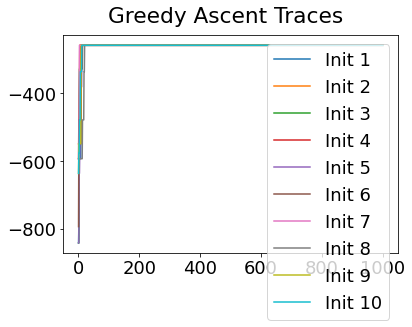
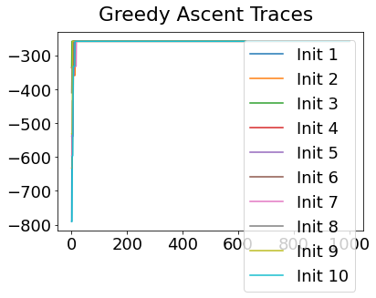
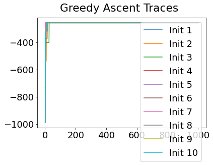
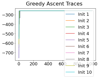
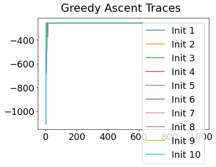
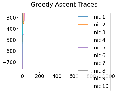
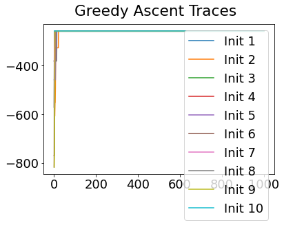
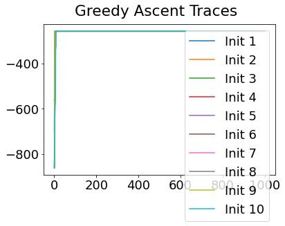
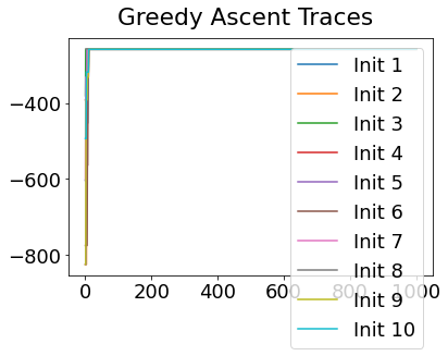
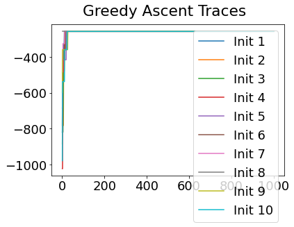
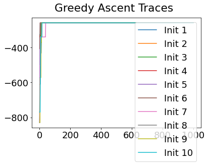
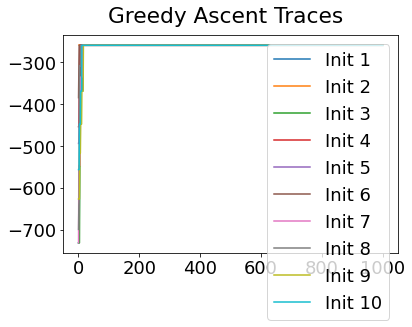
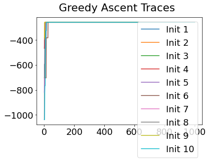
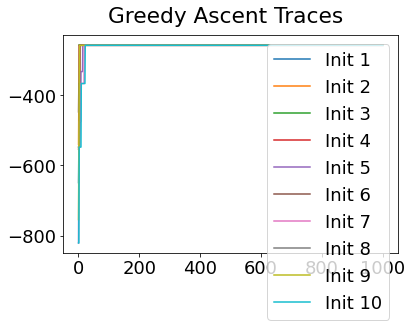
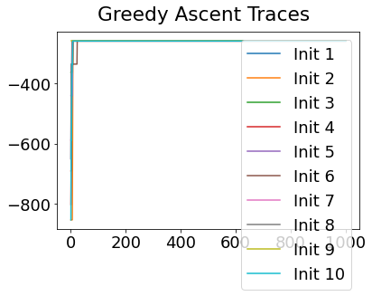
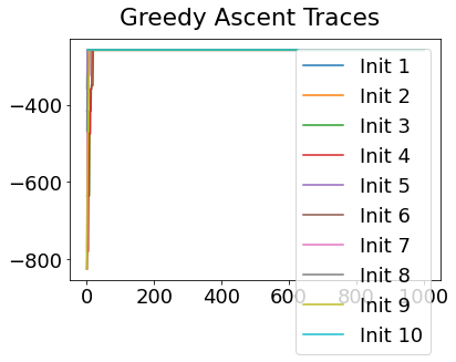
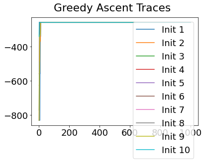
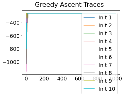
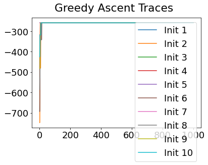
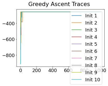
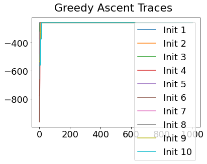
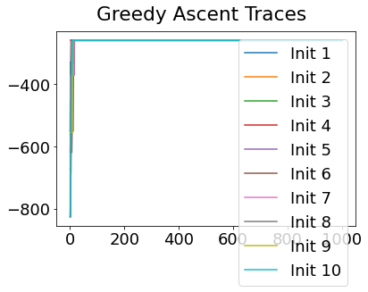
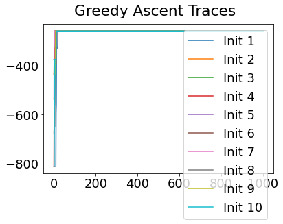
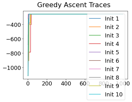
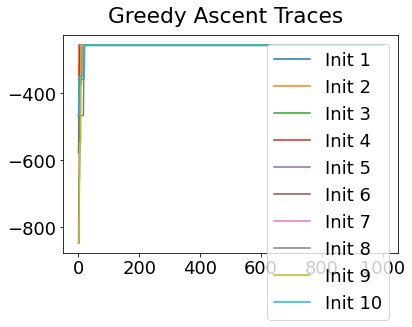
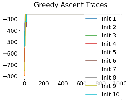
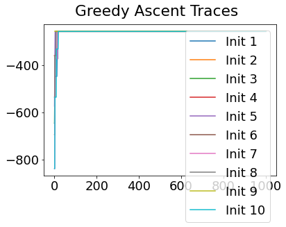
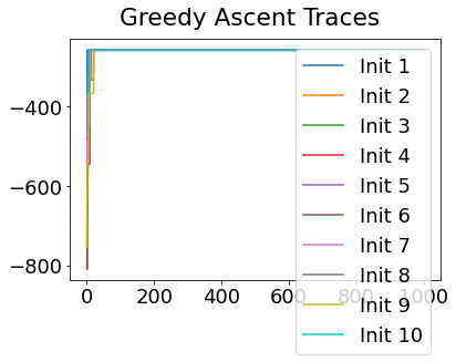
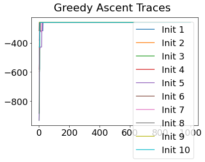
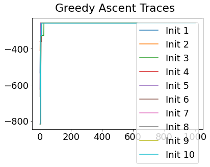
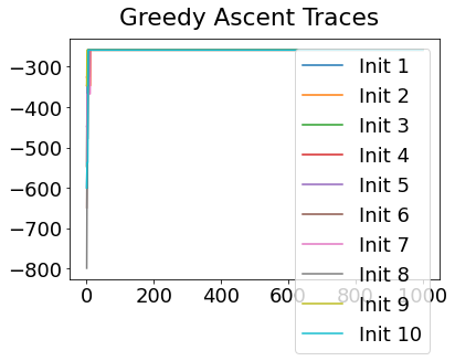
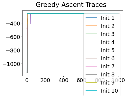
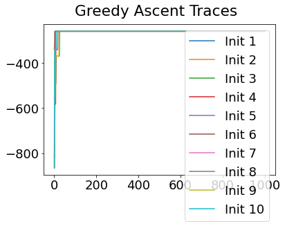
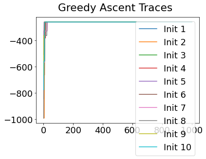
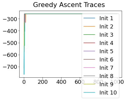
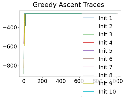
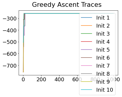
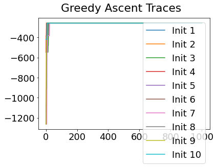
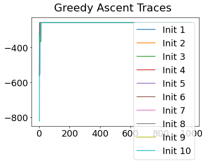

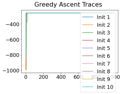
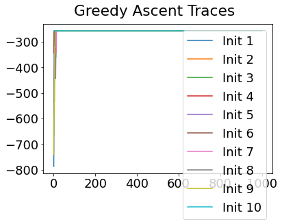
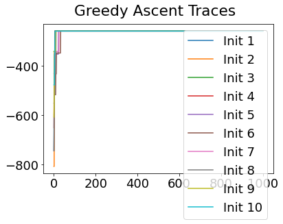
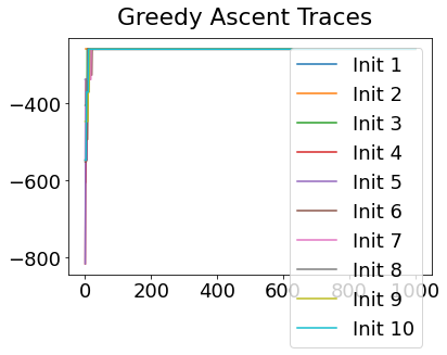
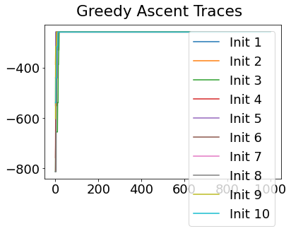
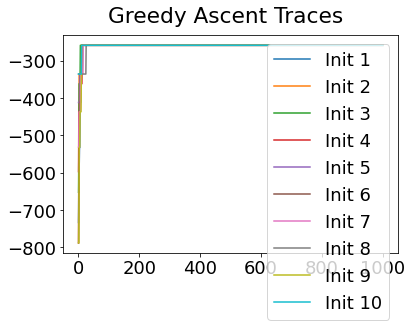
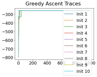
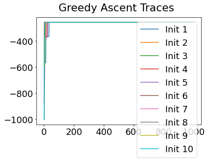
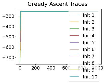
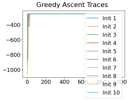
# Yet another convenience function
def extract_pvd(ml_order,samples):
    if type(ml_order) is list:
        #* List of PVDs from cross-validation/bootstrapping
        n_ = len(ml_order[0])
        pvd = np.zeros((n_,n_))
        #all_orders = np.array(ml_order)
        if type(samples[0]) is list:
            #* 10-fold CV returns MCMC samples for each fold separately in a list - concatenate them here
            all_samples = list(itertools.chain.from_iterable(samples))
        else:
            #* Bootstrapping returns MCMC samples pre-concatenated
            all_samples = samples
        all_orders = np.array([x.ordering for x in all_samples])
        for i in range(n_):
            pvd[i, :] = np.sum(all_orders == ml_order[0][i], axis=0)
        #pvd_cv, cv_rank = reorder_PVD_average_ranking(PVD=pvd)
        pvd, rank = reorder_PVD(pvd)
        seq = [ml_order[0][i] for i in rank]
    else:
        #* Single PVD (ML results)
        n_ = len(ml_order)
        pvd = np.zeros((n_,n_))
        samples_ = np.array([x.ordering for x in samples])
        seq = ml_order
        for i in range(n_):
            pvd[i, :] = np.sum(samples_ == seq[i], axis=0)
    return pvd, seq
#* Plot EBM (PVD)
pvd_rcv, seq_rcv = extract_pvd(ml_order=seqs_rcv,samples=mcmc_samples_rcv)
reorder_rcv = np.argsort(seq_rcv)
pvd_rcv_ = pvd_rcv[:][reorder_rcv]

fig, ax = plt.subplots(1,1,figsize=(9, 6),sharey=False)
labels = e_labels
labels_ = [labels[i].replace('TOTAL','').replace('TOT','').replace('-detrended','') for i in seq_rcv]
ax.imshow(pvd_rcv_[:][seq_rcv], interpolation='nearest', cmap='Oranges')
# ax.set_title('Cross-Validation',fontsize=24)

n_biomarkers = pvd_rcv.shape[0]
stp = 1
fs = 14
tick_marks_x = np.arange(0,n_biomarkers,stp)
x_labs = range(1, n_biomarkers+1,stp)
ax.set_xticks(tick_marks_x)
ax.set_xticklabels(x_labs, rotation=0,fontsize=fs)
tick_marks_y = np.arange(n_biomarkers)
ax.set_yticks(tick_marks_y+0)
ax.tick_params(axis='y',color='w')
labels_trimmed = [x[2:].replace('_', ' ') if x.startswith('p_') else x.replace('_', ' ') for x in labels_]
ax.set_yticklabels(labels_trimmed,#,np.array(labels_trimmed, dtype='object')[seq_],
                   rotation=0, #ha='right',
                   rotation_mode='anchor',
                   fontsize=18)
# ax.set_ylabel('Instrument', fontsize=28)
ax.set_xlabel('Sequence', fontsize=22)
Text(0.5, 0, 'Sequence')
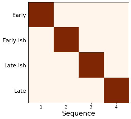
If running on real data, you might consider staging your participant data using the cross-validated model (above uses the maximum-likleihood model which can be overconfident). Then you might re-run the CV.