Disease Course Mapping#
by Igor Koval
Disease Course Mapping in a nutshell
Neurodegenerative disease progresses over periods of time longer than the usual individual observations and with an important inter-individual variability. It directly prevents to straightforwardly disentangle a reference disease progression from its manifestation at an individual level.
For that purpose, we have developed a technique called Disease Course Mapping. Its aim is to estimate, both spatially and temporally, a unified spectrum of disease progression from a population. It directly allows to :
describe the average progression (along with its variability) of the biomarkers over the entire course of the disease
position any individual onto this map to precisely characterize the patients trajectory and predict his current and future stages
Longitudinal data Non-linear Mixed-effects model Description of disease progression Personalized staging & prediction
A picture is worth a thousand words#
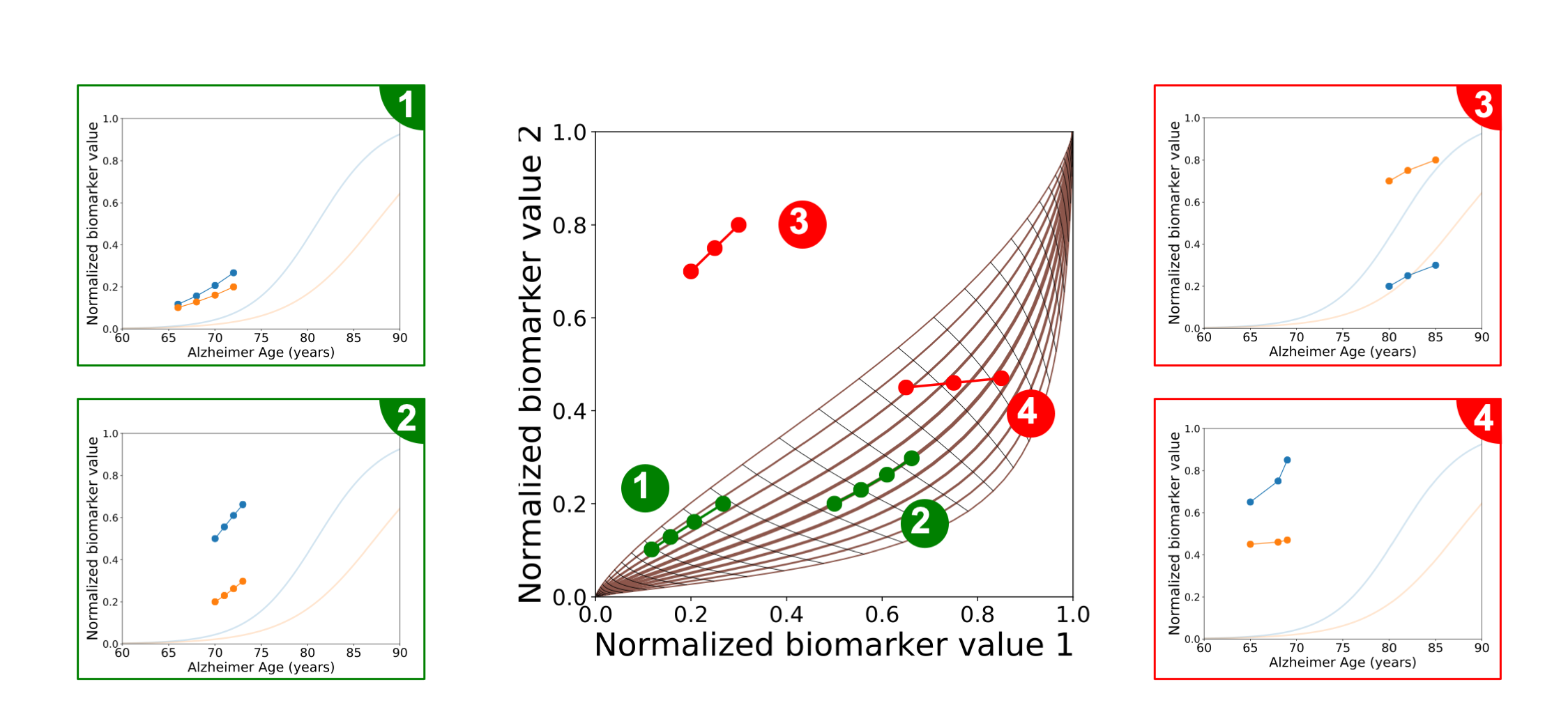
Fig. 2 Disease Course Mapping.#
The central panel corresponds to the progression of two biomarkers (x and y axis) across the course of a neurodegenerative disease. Each curve represents the progression of these biomarkers over time, from [0, 0] to [1, 1]. The central curve corresponds to the average progression whose temporal representation is represented by the two idealized blue and orange curves on the four subpanels. Each point on the mapping corresponds to the value of two biomarkers measured at any visit. The repetition of visits therefore characterizes the positioning of a patient onto the disease progression spectrum. Its variability, reflected by the envelop around the average progression as well as the orientation of the curves that corresponds to the temporal trajectories, perfectly distinguishes likely individual progressions (green subpanels) from the one that do no appear in practice (red subpanels).
Model description#
Input data
We here consider longitudinal data, i.e. patients with multiple visits along time, each corresponding to multiple observations : cognitive tests, neuropsychological assessments, medical imaging features, etc.
Attention
For the sake of clarity, in the following, we consider two biomarkers that have been normalized such that a value of 0 corresponds to normal (i.e. control) stages where 1 corresponds to pathological stages.
The aim of the model is to describe the progression of the biomarkers across the course of the disease. Let’s here assume that it corresponds to two idealized logistic curves as shown on Fig. 3. Given this average progression, how is it related to the observations of any new subject?
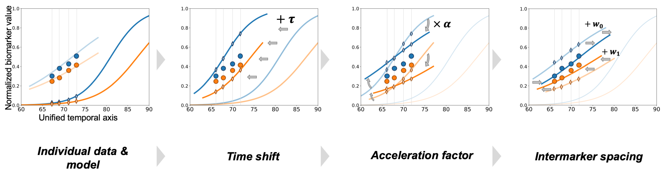
Fig. 3 The individual trajectory corresponds to the average disease progression that has been (i) shifted thanks to the time shift, (ii) decelerated thanks to the acceleration factor, and, (iii) reordered thanks to the inter-marker spacing.#
As shown on Fig. 3, we consider that the individual observations are variation of the average progressions in the sense that they derive from the mean biomarker trajectories, based on three subject-specific parameters:
The time-shift\(\tau\)It shifts the disease onset by a given number of years. For instance, a time-shift of 7 delays the entire disease progression of 7 years. \(\tau > 0\) corresponds to disease progression that are later than the average one, while \(\tau < 0\) corresponds to earlier than average progression.
acceleration factor\(\alpha\)It accelerates (\(\alpha > 1\)) or deccelerate (\(\alpha < 1\)) the overall disease progression, i.e. it changes the slope of the logistic curves
inter-marker spacing\(\omega\)It accounts for the fact that the ordering of the event (i.e. biomarker progression) might differ within the population, therefore to each patient corresponds a given sequence of events described by the vector \(\omega\) that shifts each logistic curve. [Note: To ensure identifiability with the parameter \(\tau\), we enforce \(\sum \omega_k = 0\) ].
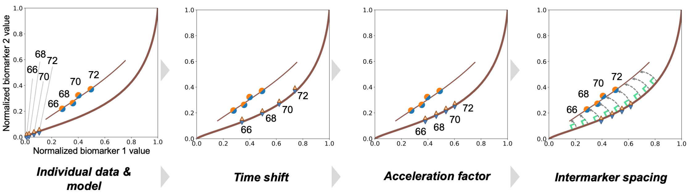
Fig. 4 Variation of the average trajectory to the individual data in the Disease Mapping space.#
The procedure that allows to derive the average trajectory can also be shown in the space of the biomarker, as shown on Fig. 4. It shows how the average progression is changed to fit the individual data - and vice-versa.
Though, a question still holds
How do we first estimate the average progression of the biomarkers from which any individual observations derive?
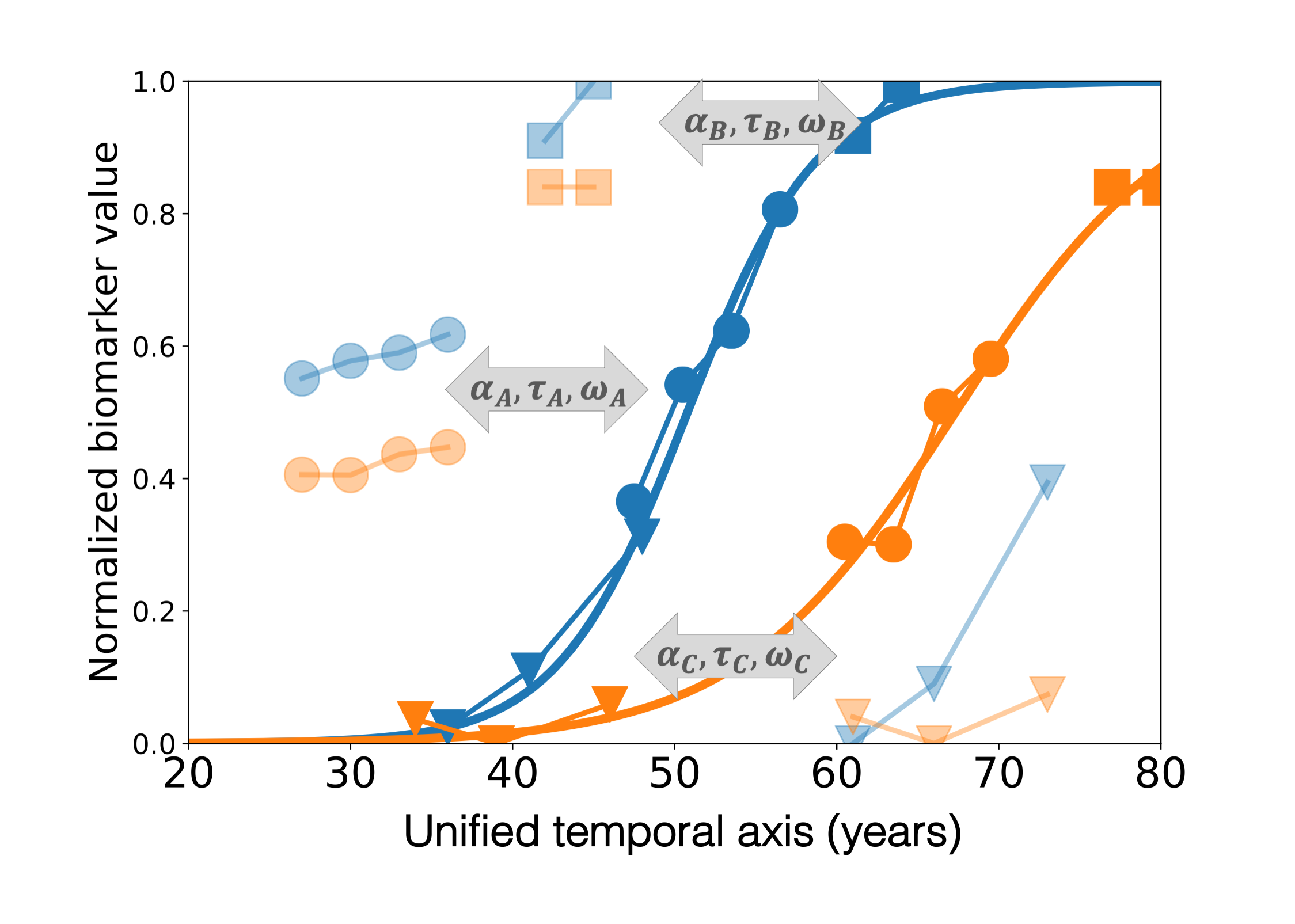
Fig. 5 Model estimation#
In practice, the average model of progression and the individual parameters are jointly estimated such that:
the variation of the mean trajectory fits the individual data (stochastic maximum likelihood estimation)
the individual parameters are considered as random variables whose mean corresponds to the average trajectory (mixed-effect model)
This procedure is sketched on Fig. 5 which shows that the average model corresponds to the recombination of the short-term individual measurements onto a long-term disease progression that spans different disease stages.
Then, once the model has been estimated, the estimation of the parameter of a new patient given this data corresponds to an optimization procedure, that under-the-hoods minimize the fit to the data and a regularization term over the individual parameters that follow normal distributions.
Note
As we derive a continuous model to fit the individual data, we can predict the future biomarkers values base on the patient observation as shown on Fig. 6. Such procedure can be done from a baseline visit only, and, has shown to be accurate (up to the noise level of the data) up to 5 years in advance.
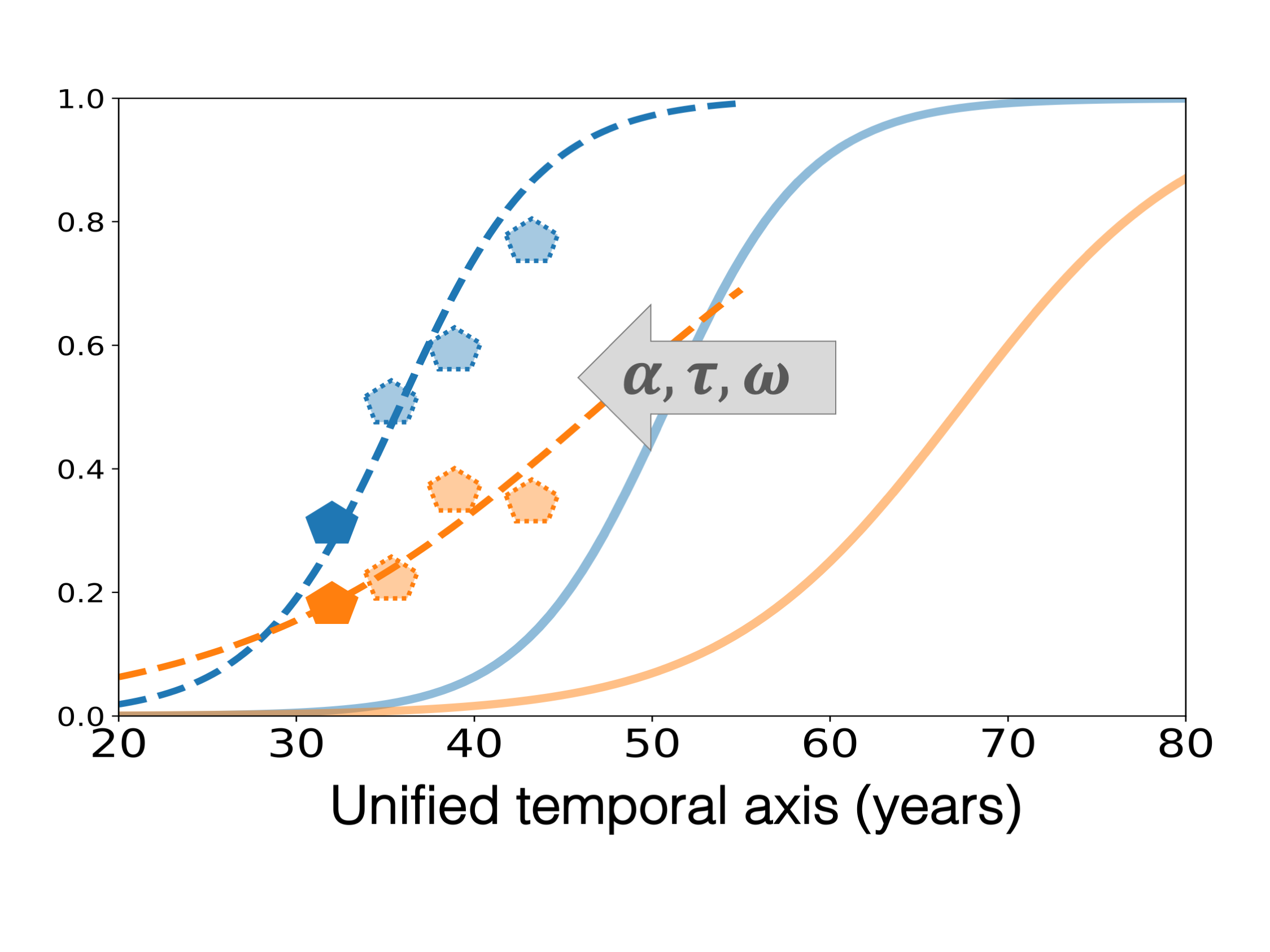
Fig. 6 The personalization of the average trajectory to the individual data allows to predict the future values of the different biomarkers.#
Disease Course Mapping as a software
Interested by this model? You want to test it on your own data?
It is made very easy thanks to the Leaspy software package. Give a look at the tutorials here.
Software Python package Open source Tutorials
References#
More detailed explanations about the models themselves and about the estimation procedure can be found in the following articles :
Mathematical Framework
A Bayesian mixed-effects model to learn trajectories of changes from repeated manifold-valued observations. Jean-Baptiste Schiratti, Stéphanie Allassonnière, Olivier Colliot, and Stanley Durrleman. The Journal of Machine Learning Research, 18:1–33, December 2017.
Model instantiations
Application to imaging data: Statistical learning of spatiotemporal patterns from longitudinal manifold-valued networks. I. Koval, J.-B. Schiratti, A. Routier, M. Bacci, O. Colliot, S. Allassonnière and S. Durrleman. MICCAI, September 2017.
Application to imaging data: Spatiotemporal Propagation of the Cortical Atrophy: Population and Individual Patterns. Igor Koval, Jean-Baptiste Schiratti, Alexandre Routier, Michael Bacci, Olivier Colliot, Stéphanie Allassonnière, and Stanley Durrleman. Front Neurol. 2018 May 4;9:235.
Application to data with missing values: Learning disease progression models with longitudinal data and missing values. R. Couronne, M. Vidailhet, JC. Corvol, S. Lehéricy, S. Durrleman
Applications
Applications for Alzheimer’s Disease progression: AD Course Map charts Alzheimer’s disease progression, I. Koval, A. Bone, M. Louis, S. Bottani, A. Marcoux, J. Samper-Gonzalez, N. Burgos, B. Charlier, A. Bertrand, S. Epelbaum, O. Colliot, S. Allassonniere & S. Durrleman, Under review.
Application to better include patients in clinical trials for Huntington disease: Machine learning spots the time to treat Huntington disease, I. Koval, T. Dighiero-Brecht, A. Tobin, S. Tabrizi, R. Scahill, S. Durrleman & A. Durr. Under review.
Website & Code
Digital Brain website: website related to the application of the model for Alzheimer’s disease
Gitlab repository : Leaspy Software, used for all the previous experiments.
Contacts#
Igor Koval (See Contributors)
Stanley Durrleman http://www.aramislab.fr/