Linear Mixed-effects Models¶

Welcome for the first practical session of the day !

Objectives :¶

Get a better idea of medical data, especially longitudinal ones
Understand mixed-effects models
Get a taste of state-of-the-art techniques

The set-up¶

If you have followed the installation details carefully, you should

be running this notebook in the leaspy_tutorial conda environment (be sure that the kernel you are using is leaspy_tutorial => check Kernel above)
having all the needed packages already install

💬 Question 1 💬 Run the following command lines

import os
import sys

import pandas as pd
import numpy as np
from scipy import stats

import matplotlib.pyplot as plt
import seaborn as sns
%matplotlib inline

Part I: The data¶

We import a functional medical imaging dataset. We have extracted, for each timepoint, the average value of the metabolic activity of the putamen. This brain region is commonly damaged by Parkinson’s disease.

IMPORTANT: The values have been normalized such that a normal value is zero and a very abrnomal value is one.

💬 Question 2 💬 Run the following cell and look at the head of the dataframe to better understand what the data are.

from leaspy.datasets import Loader
df = Loader.load_dataset('parkinson-putamen-train_and_test')

# To complete

# –––––––––––––––– #
# –––– Answer –––– #
# –––––––––––––––– #

df.head()

			PUTAMEN
ID	TIME	SPLIT
GS-001	71.354607	train	0.728492
	71.554604	train	0.735620
	72.054604	train	0.757409
	73.054604	train	0.800754
	73.554604	train	0.870756

ℹ️ Information ℹ️ The SPLIT column already distinguishes the train and test data.

💬 Question 3 💬 Describe the target variable PUTAMEN and the explicative variable TIME. You can plot:

Sample size
Mean, std
Min & max values
Quantiles

# To complete

# –––––––––––––––– #
# –––– Answer –––– #
# –––––––––––––––– #

df.reset_index().describe().round(2).T

	count	mean	std	min	25%	50%	75%	max
TIME	1997.0	65.37	10.05	33.14	58.66	66.48	72.06	91.24
PUTAMEN	1997.0	0.71	0.10	0.35	0.64	0.71	0.77	0.96

💬 Question 4 💬 From this value, what can you say about the disease stage of the population?

Your answer: …

Answer: The median and mean value is 0.71, so the average disease stage is high for these subjects.

💬 Question 5 💬 Display the data, where the Putamen (y-axis) is plot with respect to the Time (x-axis)

# To complete

# –––––––––––––––– #
# –––– Answer –––– #
# –––––––––––––––– #

sns.set_style('whitegrid')
plt.figure(figsize=(14,6))
sns.scatterplot(data=df.xs('train', level='SPLIT').reset_index(), 
                x='TIME', y='PUTAMEN', alpha=.5, s=60)
plt.title('PUTAMEN - Raw data')
plt.show()

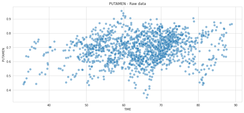
⚡ Remark ⚡ At first look, the PUTAMEN values do not seem highly correlated to TIME.

Part II: Linear Regression¶

As we are some pro ML players, let’s make some predictions : let’s try to predict the putamen value based on the time alone.

💬 Question 6 💬 Store the train and test data in df_train and df_test

# To complete

# –––––––––––––––– #
# –––– Answer –––– #
# –––––––––––––––– #

pds = pd.IndexSlice
df_train = df.loc[pds[:, :, 'train']].copy()  # one possibility
df_test = df.xs('test', level='SPLIT').copy()  # an other one

💬 Question 7 💬 Run the linear reagression that is in scipy.

Be carefull, you have to train it only with the train set!

x = # Complete with the appropriate data
y = # Complete with the appropriate data

slope, intercept, r_value, p_value, std_err = stats.linregress(x, y)

# –––––––––––––––– #
# –––– Answer –––– #
# –––––––––––––––– #

x = df_train.index.get_level_values('TIME').values
y = df_train['PUTAMEN'].values

slope, intercept, r_value, p_value, std_err = stats.linregress(x, y)

ℹ️ Information ℹ️ To run the notebook smoothly, you must comply to the following rules: we are going to try different models to predict the putamen values based on each observation.

We will store the results in the dataframe df such that :

ID	TIME	SPLIT	PUTAMEN	Model 1	Model 2	…
GS-001	74.4	train	0.78	0.93	0.75	…
GS-003	75.4	train	0.44	0.84	0.46	…
GS-018	51.8	test	0.71	0.73	0.78	…
GS-056	89.2	train	0.76	0.56	0.61	…

This will ease the comparison of the models.

⚡ Remark ⚡ No need to add these predictions to df_train and df_test. You should be able to easily run the notebook by keeping df_train the way it is while appending the results in df.

💬 Question 8 💬 Add the predictions done by the linear regression in the column Linear Regression

df['Linear Regression'] = # Your code here

# –––––––––––––––– #
# –––– Answer –––– #
# –––––––––––––––– #

df['Linear Regression'] = intercept + slope * df.index.get_level_values('TIME')

ℹ️ Information ℹ️ Let’s introduce an object and a fonction that will be used to compare the models:

overall_results will be the dataframe that stores the root mean square error on the train and test set for the different models
compute_rmse_train_test is the function that given the dataframe df and a model_name (Linear Regression for instance), compute the mean absolute error on the train and test set and stores it in overall_results

💬 Question 9 💬 Run the following cell to see the results

overall_results = pd.DataFrame({'train': [], 'test': []})  


def compute_rmse(df, model_name):
    """Compute RMSE between PUTAMEN column and the <model_name> column of df"""
    y = df['PUTAMEN']
    y_hat = df[model_name]
    diff = y - y_hat
    return np.sqrt(np.mean(diff * diff))


def compute_rmse_train_test(df, overall_results, model_name):
    """Inplace modification of <overall_results>"""
    overall_results.loc[model_name, 'train'] = compute_rmse(df.xs('train', level='SPLIT'), model_name)
    overall_results.loc[model_name, 'test'] = compute_rmse(df.xs('test', level='SPLIT'), model_name)

compute_rmse_train_test(df, overall_results, 'Linear Regression')
overall_results

	train	test
Linear Regression	0.091403	0.10213

⚡ Remark ⚡ The RMSE is higher on the test set as on the train set

Let’s look at what we are doing by plotting the data and the linear regression. Throughout the notebook, we will use the function plot_individuals that, given a subset of IDs and a model name (as stored in the df dataframe) plots the individual data and their prediction

💬 Question 10 💬 Use the following cell.

def get_title(overall_results, model_name):
    """Precise model's name and its RMSE train & test"""
    rmse_train = overall_results.loc[model_name, 'train']
    rmse_test = overall_results.loc[model_name, 'test']
    title = f'PUTAMEN - Raw data vs {model_name:s}\n'
    title += r'$RMSE_{train}$ = %.3f     $RMSE_{test}$ = %.3f' % (rmse_train, rmse_test)
    return title

    
def plot_individuals(df, overall_results, model_name, **kwargs):
    # ---- Input manager
    kind = kwargs.get('kind', 'lines')
    sublist = kwargs.get('sublist', None)
    highlight_test = kwargs.get('highlight_test', True)
    ax = kwargs.get('ax', None)
    
    if ax is None:
        fig, ax = plt.subplots(figsize=(14, 6))
    else:
        plt.figure(figsize=(14, 6))
    
    # ---- Select subjects
    if sublist is None:
        sublist = df.index.unique('ID')
        
    # ---- If too many subject, do not display them in the legend
    display_id_legend = len(sublist) <= 10
    
    # ---- Plot
    if kind == 'scatter':
        # -- Used for Linear Regression
        sns.scatterplot(data=df.reset_index(), x='TIME', y='PUTAMEN', alpha=.5, 
                        s=60, label='Observations', ax=ax)
        ax.plot(df.index.get_level_values('TIME').values,
                df[model_name].values, 
                label=model_name, c='C1')
        ax.legend(title='LABEL')
        if highlight_test:
            test = df.xs('test', level='SPLIT').loc[sublist].reset_index()
            sns.scatterplot(data=test, x='TIME', y='PUTAMEN', legend=None, ax=ax)
        
    elif kind == 'lines':
        # -- Used for the other models
        # - Stack observations & reconstructions by the model
        df_stacked = df[['PUTAMEN', model_name]].copy()
        df_stacked.rename(columns={'PUTAMEN': 'Observations'}, inplace=True)
        df_stacked = df_stacked.stack().reset_index().set_index(['ID', 'SPLIT'])
        df_stacked.columns = ['TIME', 'LABEL', 'PUTAMEN']
        
        # - Plot
        sns.lineplot(data=df_stacked.loc[sublist], 
                     x='TIME', y='PUTAMEN', hue='ID', style='LABEL', 
                     legend=display_id_legend, ax=ax)
        if highlight_test:
            test = df.xs('test', level='SPLIT').loc[sublist].reset_index()
            sns.scatterplot(data=test, x='TIME', y='PUTAMEN', hue='ID', legend=None, ax=ax)
        if display_id_legend:
            ax.legend(title='LABEL', bbox_to_anchor=(1.05, 1), loc='upper left')
    else:
        raise ValueError('<kind> input accept only "scatter" and "lines".'
                         f' You gave {kind}')
        
    ax.set_title(get_title(overall_results, model_name))
    return ax
    
plot_individuals(df, overall_results, 'Linear Regression', 
                 kind='scatter', highlight_test=False)
plt.show()

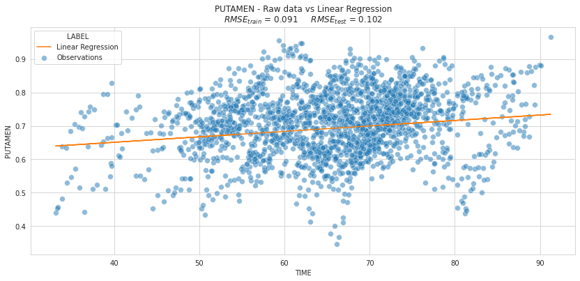
Is the previous plot relevant to assess the quality of our model?

We will answer this question in the following cells:

Part III: The longitudinal aspect¶

💬 Question 11 💬 Run the cell to have a better understanding of your data:

plot_individuals(df, overall_results, 'Linear Regression', 
                 kind='lines', highlight_test=True)
plt.title('Longitudinal aspect')
plt.show()

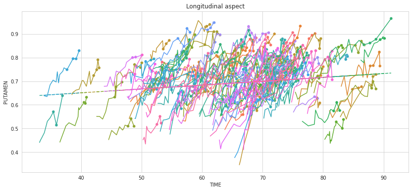
The test data are highlited with dots. 💬 Question 12 💬 What are actually the test data ?

Your answer: …

💬 Question 13 💬Why does the global linear model not describe the temporal evolution of the variable?

Your answer: …

PART IV: Indivual Linear Regressions¶

ℹ️ Information ℹ️ In fact, this is not the best idea to have one general linear regression. Because we do not benefit from indiviudal information. Therefore, let’s do one linear regression per individual

💬 Question 14 💬 Look at what this function is doing and at the result

individual_parameters = pd.DataFrame({'INTERCEPT': [], 'SLOPE': []})

subject_idx = 'GS-194'

def compute_individual_parameters(df, subject_idx):
    df_patient = df.loc[subject_idx]
    
    x = df_patient.index.get_level_values('TIME').values
    y = df_patient['PUTAMEN'].values
    
    # -- Linear regression
    slope, intercept, _, _, _ = stats.linregress(x, y)
    
    return intercept, slope

individual_parameters.loc[subject_idx] = compute_individual_parameters(df_train, subject_idx)

individual_parameters

	INTERCEPT	SLOPE
GS-194	0.025188	-0.807941

💬 Question 15 💬 Apply the function to everyone

# Your answer

# –––––––––––––––– #
# –––– Answer –––– #
# –––––––––––––––– #


for subject_idx in df_train.index.unique('ID'):
   
    slope, intercept = compute_individual_parameters(df_train, subject_idx)
    individual_parameters.loc[subject_idx] = (intercept, slope)
    
individual_parameters.head()

	INTERCEPT	SLOPE
GS-194	-0.807941	0.025188
GS-001	-2.946305	0.051464
GS-002	-0.252949	0.018643
GS-003	0.517972	0.003816
GS-004	-1.076280	0.025680

💬 Question 16 💬 Now append the result of the model in df using the function below.

⚡ Remark ⚡ Take a close look at what we are doing cause we will use the same syntax if other questions.

def compute_individual_reconstruction(x, parameters):
    
    subject_idx = x.name[0]
    
    slope = parameters.loc[subject_idx]['SLOPE']
    intercept = parameters.loc[subject_idx]['INTERCEPT']
    
    time = x.name[1]
    
    return intercept + slope * time
    
df['Individual Linear Regression'] = df.apply(
    lambda x: compute_individual_reconstruction(x, individual_parameters), axis=1)

💬 Question 17 💬 Use the compute_train_test_mean_absolute_error function to get the train and test errors and compare the two models.

# Your code here

# –––––––––––––––– #
# –––– Answer –––– #
# –––––––––––––––– #

compute_rmse_train_test(df, overall_results, 'Individual Linear Regression')
overall_results

	train	test
Linear Regression	0.091403	0.102130
Individual Linear Regression	0.017825	0.032197

We clearly see that the RMSE is much better! 💬 Question 18 💬 Create a list with the five patients having the more visits and the five patients having the less visits, then use plot_individuals function to display their observations and reconstructions by the model Hint : use the keyword sublist

# sublist = # TODO
# plot_individuals(df, overall_results, model_name, sublist=sublist)

# –––––––––––––––– #
# –––– Answer –––– #
# –––––––––––––––– #

visits_per_subjects = df.groupby(df.index.get_level_values('ID')).count().sort_values('PUTAMEN')
sublist = visits_per_subjects.tail(5).index.tolist()
sublist += visits_per_subjects.head(5).index.tolist()

plot_individuals(df, overall_results, 'Individual Linear Regression', sublist=sublist)
plt.show()

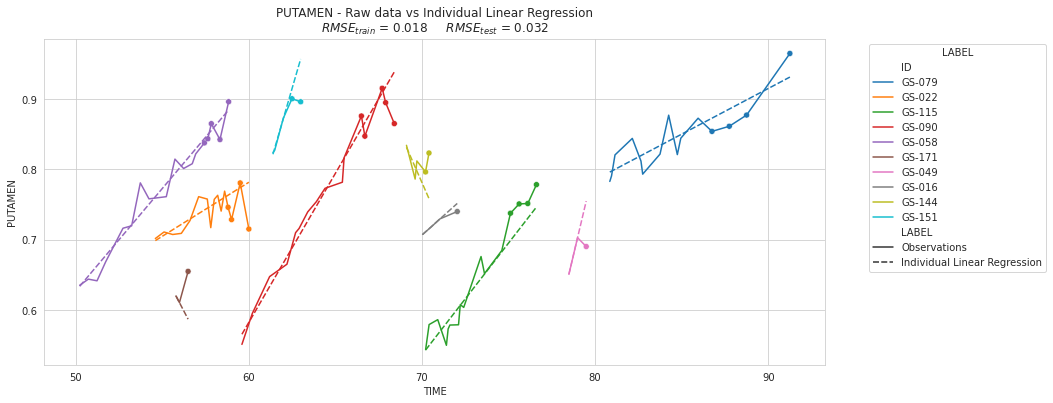
💬 Question 19 💬 Explain why $RMSE_{test} >> RMSE_{train}$:

Your answer: …

Answer: the LM overfit for patients with only few data

Part V : Linear Mixed effects Model with `statsmodels`¶

With the previous method, we made a significant improvement. However, we suffer fro an overfitting problem. Let’s see what a mixed effect model can do for us!

Run a LMM with `statsmodels`¶

ℹ️ Information ℹ️ We will use the statsmodel package to run a Linear Mixed Effect Model (LMM or LMEM in the literature).

💬 Question 20 💬 Load the following lines to import the packages

import statsmodels.api as sm
import statsmodels.formula.api as smf
from statsmodels.regression.mixed_linear_model import MixedLMParams

Statsmodels contains several API to create a model. For the ones familiar with R, you will be here in a familiar ground with the formula API.

formula='PUTAMEN ~ TIME + 1' means that you want to explain PUTAMEN with TIME and an intercept
groups="ID" means that you want random effect for all levels of ID
re_formula="~TIME + 1" means that you want a random intercept and a random slope for TIME

If you go back to the equation you get : $ PUTAMEN_{id,time} = \underbrace{\alpha*TIME_{id,time} + \beta}_\text{formula} + \underbrace{\alpha_{id}*TIME_{id,time} + \beta_{id}}_\text{re_formula}$

💬 Question 21 💬 Let’s try a very naive run:

lmm = smf.mixedlm(formula='PUTAMEN ~ 1 + TIME', 
                  data=df_train.reset_index(), 
                  groups="ID", re_formula="~ 1 + TIME").fit()
lmm.summary()

/home/juliette.ortholand/miniconda3/envs/leaspype/lib/python3.8/site-packages/statsmodels/base/model.py:566: ConvergenceWarning: Maximum Likelihood optimization failed to converge. Check mle_retvals
  warnings.warn("Maximum Likelihood optimization failed to "
/home/juliette.ortholand/miniconda3/envs/leaspype/lib/python3.8/site-packages/statsmodels/regression/mixed_linear_model.py:2200: ConvergenceWarning: Retrying MixedLM optimization with lbfgs
  warnings.warn(
/home/juliette.ortholand/miniconda3/envs/leaspype/lib/python3.8/site-packages/statsmodels/regression/mixed_linear_model.py:2237: ConvergenceWarning: The MLE may be on the boundary of the parameter space.
  warnings.warn(msg, ConvergenceWarning)

Model:	MixedLM	Dependent Variable:	PUTAMEN
No. Observations:	1415	Method:	REML
No. Groups:	200	Scale:	0.0007
Min. group size:	2	Log-Likelihood:	2497.0458
Max. group size:	13	Converged:	Yes
Mean group size:	7.1

	Coef.	Std.Err.	z	P>\|z\|	[0.025	0.975]
Intercept	-0.685	0.044	-15.644	0.000	-0.771	-0.599
TIME	0.022	0.001	29.528	0.000	0.020	0.023
ID Var	0.003	0.259
ID x TIME Cov	0.000	0.005
TIME Var	0.000	0.000

⚡ Remark ⚡ Let’s skip the different warning for now and see what happens if we ignore it

Let’s try and see.

💬 Question 22 💬 Run the following commands to get the intercept and slope

print(lmm.fe_params.loc['Intercept'])
print(lmm.fe_params.loc['TIME'])

-0.6848661069361888
0.021679337332944623

💬 Question 23 💬 Run the following commands to get the variation to the mean slope and intercept Example on few subject

{key: val for key, val in lmm.random_effects.items() if key in 
 ['GS-00'+str(i) for i in range(1, 4)]}

{'GS-001': ID     -0.019149
 TIME   -0.001092
 dtype: float64,
 'GS-002': ID      0.058495
 TIME    0.004182
 dtype: float64,
 'GS-003': ID     -0.011974
 TIME   -0.001002
 dtype: float64}

💬 Question 24 💬 From the fixed and random effects, compute for each subject its INTERCEPT and SLOPE:

# df_random_effects['INTERCEPT'] = # TODO
# df_random_effects['SLOPE'] = # TODO

# df_random_effects.head()

# –––––––––––––––– #
# –––– Answer –––– #
# –––––––––––––––– #

df_random_effects = pd.DataFrame.from_dict(lmm.random_effects, orient='index')
df_random_effects = df_random_effects.rename({'ID': 'Random intercept', 'TIME': 'Random slope'}, axis=1)

df_random_effects['INTERCEPT'] = df_random_effects['Random intercept'] + lmm.fe_params.loc['Intercept']
df_random_effects['SLOPE'] = df_random_effects['Random slope'] + lmm.fe_params.loc['TIME']

df_random_effects.head()

	Random intercept	Random slope	INTERCEPT	SLOPE
GS-001	-0.019149	-0.001092	-0.704015	0.020588
GS-002	0.058495	0.004182	-0.626371	0.025861
GS-003	-0.011974	-0.001002	-0.696840	0.020677
GS-004	-0.020968	-0.001529	-0.705834	0.020150
GS-005	0.006285	0.000363	-0.678581	0.022043

💬 Question 25 💬 Use the compute_individual_reconstruction function but with df_random_effects to compute the prediction with the new individual effects

df['Linear Mixed Effect Model'] = # Your code here

# –––––––––––––––– #
# –––– Answer –––– #
# –––––––––––––––– #

df['Linear Mixed Effect Model'] = df.apply(
    lambda x: compute_individual_reconstruction(x, df_random_effects), axis=1)

💬 Question 26 💬 Store the results in overall_results (thanks to compute_rmse_train_test function) and compare the models

# Your code here

# –––––––––––––––– #
# –––– Answer –––– #
# –––––––––––––––– #

compute_rmse_train_test(df, overall_results, 'Linear Mixed Effect Model')

overall_results

	train	test
Linear Regression	0.091403	0.102130
Individual Linear Regression	0.017825	0.032197
Linear Mixed Effect Model	0.024533	0.039367

⚡ Remark ⚡ The result is worse than with the previous model.

💬 Question 27 💬 What do you think happened? Let’s check it visually

# Your code here

# –––––––––––––––– #
# –––– Answer –––– #
# –––––––––––––––– #

plot_individuals(df, overall_results, 'Linear Mixed Effect Model', sublist=sublist)
plt.show()

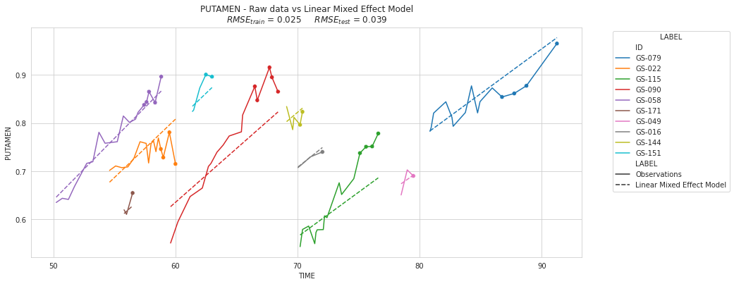
⚡ Remark ⚡ All the slopes are the same. This is related to the warning above : these are warnings are a way of alerting you that you may be in a non-standard situation. Most likely, one of your variance parameters is converging to zero. Which is the case if you have a look to time variance.

💬 Question 28 💬 Let’s rerun it by normalizing the time first. Add to df_train and df_test a renormalizing function. Be careful to normalize only with the known ages from train. Hint : Watchout to data leakage!

# Your code

df['TIME_NORMALIZED'] = # Your code

# ---- Split again train & test
df_train = df.xs('train',level='SPLIT')
df_test = df.xs('test',level='SPLIT')

# –––––––––––––––– #
# –––– Answer –––– #
# –––––––––––––––– #

# ---- We use only train data to compute mean & std
ages = df_train.index.get_level_values(1).values
age_mean = ages.mean()
age_std = ages.std()

df['TIME_NORMALIZED'] = (df.index.get_level_values('TIME') -  age_mean) / age_std

# ---- Split again train & test
df_train = df.xs('train',level='SPLIT')
df_test = df.xs('test',level='SPLIT')

💬 Question 29 💬 Rerun the previous mixed lm (some cells above) but with the TIME_NORMALIZED instead of TIME in the formula and re_formula.

# YOUR CODE

# –––––––––––––––– #
# –––– Answer –––– #
# –––––––––––––––– #


lmm = smf.mixedlm(formula='PUTAMEN ~ TIME_NORMALIZED + 1', data=df_train.reset_index(), 
                  groups="ID", re_formula="~TIME_NORMALIZED + 1").fit()

lmm.summary()

Model:	MixedLM	Dependent Variable:	PUTAMEN
No. Observations:	1415	Method:	REML
No. Groups:	200	Scale:	0.0005
Min. group size:	2	Log-Likelihood:	2629.4084
Max. group size:	13	Converged:	Yes
Mean group size:	7.1

	Coef.	Std.Err.	z	P>\|z\|	[0.025	0.975]
Intercept	0.679	0.016	43.031	0.000	0.648	0.710
TIME_NORMALIZED	0.231	0.011	20.134	0.000	0.209	0.254
ID Var	0.045	0.288
ID x TIME_NORMALIZED Cov	-0.006	0.111
TIME_NORMALIZED Var	0.017	0.126

Ahaaaaah! No warnings!

💬 Question 30 💬 Get the parameters as previously in df_random_effects_2 and store the INTERCEPT_NORMALIZED and SLOPE_NORMALIZED

# TODO

# –––––––––––––––– #
# –––– Answer –––– #
# –––––––––––––––– #


df_random_effects_2 = pd.DataFrame.from_dict(lmm.random_effects, orient='index')
df_random_effects_2 = df_random_effects_2.rename({'ID': 'Random intercept', 'TIME_NORMALIZED': 'Random slope'},
                                                 axis=1)


df_random_effects_2['INTERCEPT_NORMALIZED'] = df_random_effects_2['Random intercept'] + \
                                              lmm.fe_params.loc['Intercept']
df_random_effects_2['SLOPE_NORMALIZED'] = df_random_effects_2['Random slope'] + \
                                          lmm.fe_params.loc['TIME_NORMALIZED']

df_random_effects_2.head()

	Random intercept	Random slope	INTERCEPT_NORMALIZED	SLOPE_NORMALIZED
GS-001	-0.222614	0.185999	0.456428	0.417479
GS-002	0.233375	-0.075922	0.912417	0.155558
GS-003	0.009845	-0.091712	0.688887	0.139767
GS-004	-0.093862	0.017902	0.585179	0.249382
GS-005	0.055686	-0.050411	0.734728	0.181068

Here, we computed

\[ y = SLOPE_{normalized} * TIME_{normalized} + INTERCEPT_{normalized} \]

which corresponds to

\[ y = SLOPE_{normalized} * \frac{(TIME - \mu(ages))}{ \sigma_{ages}} + INTERCEPT_{normalized} \]

which is :

\[ y = SLOPE * TIME + INTERCEPT \]

where $$SLOPE = \frac{SLOPE_{normalized}}{ std_{ages}}$$ and $$INTERCEPT = INTERCEPT_{normalized} - \frac{SLOPE_{normalized} * mean_{ages}}{std_{ages}}$$

💬 Question 31 💬 From INTERCEPT_NORMALIZED & SLOPE_NORMALIZED, compute for each subject its INTERCEPT and SLOPE:

parameters['GS-001'] 
>>> {'INTERCEPT': ..., 'SLOPE': ...}

# YOUR CODE

# –––––––––––––––– #
# –––– Answer –––– #
# –––––––––––––––– #

df_random_effects_2['SLOPE'] = df_random_effects_2['SLOPE_NORMALIZED'] / age_std
df_random_effects_2['INTERCEPT'] = df_random_effects_2['INTERCEPT_NORMALIZED'] -\
                                   (df_random_effects_2['SLOPE_NORMALIZED'] * age_mean)/age_std

💬 Question 32 💬 Use the compute_individual_reconstruction function but with df_random_effects_2 to compute the prediction with the new individual effects

# Your code

# –––––––––––––––– #
# –––– Answer –––– #
# –––––––––––––––– #

df['Linear Mixed Effect Model - V2'] = df.apply(
    lambda x: compute_individual_reconstruction(x, df_random_effects_2), axis=1)

💬 Question 33 💬 Store the results in overall_results (thanks to compute_rmse_train_test function) and compare the models

# Your code

# –––––––––––––––– #
# –––– Answer –––– #
# –––––––––––––––– #

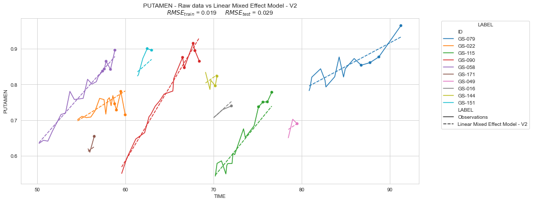
compute_rmse_train_test(df, overall_results, 'Linear Mixed Effect Model - V2')

overall_results

	train	test
Linear Regression	0.091403	0.102130
Individual Linear Regression	0.017825	0.032197
Linear Mixed Effect Model	0.024533	0.039367
Linear Mixed Effect Model - V2	0.019081	0.028939

The RMSE is much better!

💬 Question 34 💬 Display the subjects of sublist :

# Your code

# –––––––––––––––– #
# –––– Answer –––– #
# –––––––––––––––– #

plot_individuals(df, overall_results, 'Linear Mixed Effect Model - V2', sublist=sublist)
plt.show()

💬 Question 35 💬 What is the main advantage of a Linear Mixed-effects Model compared to multiple Linear Models ?

Your answer…

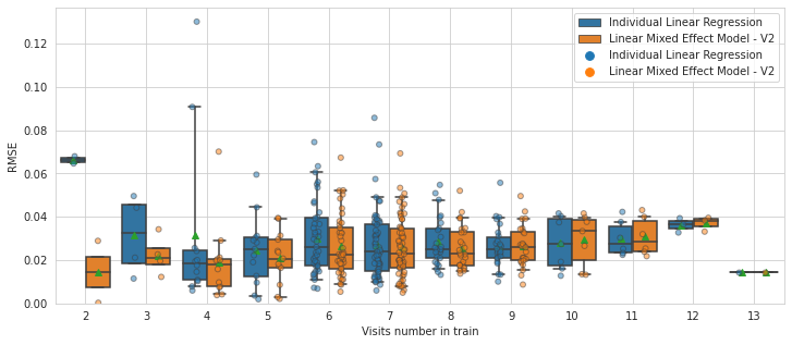
💬 Question 36 💬 Let’s check the average RMSE per subject depending of the number of timepoints per subjects:

models = ['Individual Linear Regression', 'Linear Mixed Effect Model - V2']


def plot_rmse_by_number_of_visit(models, df=df):
    rmse = df[models].copy()
    rmse.columns.names = ['MODEL']
    rmse = rmse.stack()
    rmse = (rmse - df['PUTAMEN']) ** 2

    nbr_of_visits = rmse.xs('train',level='SPLIT').groupby(['MODEL','ID']).size()

    rmse = rmse.xs('test',level='SPLIT')
    rmse = rmse.reset_index().rename(columns={0: 'RMSE'})
    rmse = rmse.reset_index()[['ID', 'MODEL', 'RMSE']]
    rmse = rmse.groupby(['MODEL','ID']).mean() ** .5
    rmse['Visits number in train'] = nbr_of_visits

    plt.figure(figsize=(12, 5))
    ax = sns.boxplot(data=rmse.reset_index(), y='RMSE', 
                     x='Visits number in train', hue='MODEL', 
                     showmeans=True, whis=[5,95], showfliers=False)
    ax = sns.stripplot(data=rmse.reset_index(), y='RMSE', 
                       x='Visits number in train', hue='MODEL', 
                       dodge=True, alpha=.5, linewidth=1, ax=ax)

    plt.grid(True, axis='both')
    plt.ylim(0,None)
    plt.legend()
    return ax


plot_rmse_by_number_of_visit(models, df)
plt.show()

PART VI: A taste of the future - Linear mixed-effect model with Leaspy¶

In the next practical sessions you will learn to use the package developped by the Aramis team. Now, just to be able to compare performances you will run a few methods of leaspy in advance…

💬 Question 37 💬 Run the following cell to make the import of leaspy methods, format the data and fit a model :

# --- Import methods
from leaspy import Leaspy, Data, AlgorithmSettings

# --- Format the data
data = Data.from_dataframe(df_train[['PUTAMEN']])

# --- Fit a model
leaspy_univariate = Leaspy('univariate_linear')
settings_fit = AlgorithmSettings('mcmc_saem', progress_bar=True, seed=0)
leaspy_univariate.fit(data, settings_fit)

 ==> Setting seed to 0
|##################################################|   10000/10000 iterations
The standard deviation of the noise at the end of the calibration is:
0.0215

Calibration took: 26s

Well it’s a bit slow, but here is a joke to wait:

What did the triangle say to the circle? “You’re pointless.”

…

Okay, it was short. Here is another one:

I had an argument with a 90° angle. It turns out it was right.

💬 Question 38 💬 Run the following two cells to make the predictions:

settings_personalize = AlgorithmSettings('scipy_minimize', progress_bar=True, use_jacobian=True)

individual_parameters = leaspy_univariate.personalize(data, settings_personalize)

|##################################################|   200/200 subjects
The standard deviation of the noise at the end of the personalization is:
0.0184

Personalization scipy_minimize took: 20s

timepoints = {idx: df.loc[idx].index.get_level_values('TIME').values for idx in 
              df.index.get_level_values('ID').unique()}
estimates = leaspy_univariate.estimate(timepoints, individual_parameters)

💬 Question 39 💬 Add the predictions to df

df['Leaspy linear'] = float('nan')

for idx in df.index.unique('ID'):
    df.loc[idx, 'Leaspy linear'] = estimates[idx]

💬 Question 40 💬 Compute and add the new rmse

compute_rmse_train_test(df, overall_results, 'Leaspy linear')

overall_results

	train	test
Linear Regression	0.091403	0.102130
Individual Linear Regression	0.017825	0.032197
Linear Mixed Effect Model	0.024533	0.039367
Leaspy linear	0.018394	0.027894

💬 Question 41 💬 Display the subjects of sublist :

# Your code

# –––––––––––––––– #
# –––– Answer –––– #
# –––––––––––––––– #

plot_individuals(df, overall_results, 'Leaspy linear', sublist=sublist)
plt.show()

PART VII: A taste of the future - Non-linear mixed-effect model with Leaspy¶

Again you will use an other model of leapsy…

💬 Question 42 💬 Fit the model with the data.

leaspy_univariate = Leaspy('univariate_logistic')
settings_fit = AlgorithmSettings('mcmc_saem', progress_bar=True, seed=0)
leaspy_univariate.fit(data, settings_fit)

 ==> Setting seed to 0
|##################################################|   10000/10000 iterations
The standard deviation of the noise at the end of the calibration is:
0.0214

Calibration took: 27s

💬 Question 43 💬 Run the following two cells to make the predictions:

settings_personalize = AlgorithmSettings('scipy_minimize', progress_bar=True, use_jacobian=True)

individual_parameters = leaspy_univariate.personalize(data, settings_personalize)

|##################################################|   200/200 subjects
The standard deviation of the noise at the end of the personalization is:
0.0183

Personalization scipy_minimize took: 4s

timepoints = {idx: df.loc[idx].index.get_level_values('TIME').values for idx in 
              df.index.get_level_values('ID').unique()}
estimates = leaspy_univariate.estimate(timepoints, individual_parameters)

💬 Question 44 💬 Add the predictions to df

df['Leaspy logistic'] = float('nan')

for idx in df.index.unique('ID'):
    df.loc[idx, 'Leaspy logistic'] = estimates[idx]

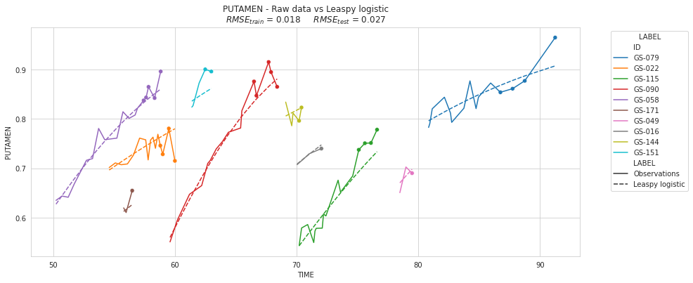
💬 Question 45 💬 Compute and add the new rmse

compute_rmse_train_test(df, overall_results, 'Leaspy logistic')

overall_results

	train	test
Linear Regression	0.091403	0.102130
Individual Linear Regression	0.017825	0.032197
Linear Mixed Effect Model	0.024533	0.039367
Leaspy linear	0.018394	0.027894
Leaspy logistic	0.018331	0.026822

💬 Question 46 💬 Display the subjects of sublist :

# Your code

# –––––––––––––––– #
# –––– Answer –––– #
# –––––––––––––––– #

plot_individuals(df, overall_results, 'Leaspy logistic', sublist=sublist)
plt.show()

💬 Question 47 💬 Check the average RMSE per subject depending of the number of timepoints per subjects

models = ['Individual Linear Regression', 
          'Linear Mixed Effect Model - V2',
          'Leaspy linear',
          'Leaspy logistic']


plot_rmse_by_number_of_visit(models, df)
plt.show()

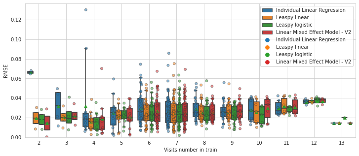
Here we clearly see that the few subjects who have less than 6 timepoints are better reconstructed with a mixed effect model!

For the fast-running Zebras: all-in-one with a more realistic split of data¶

Let’s try to split differently data so to mimic real-world applications.

We don’t want to fit again a new model every time we predict the future of a new patient. To this aim, we want to calibrate (fit) a model on a large and representative dataset once and then personalize this model to totally new individuals. We can then make forecasts about these new individuals.

The previous split was not taking into account this constraint and this extra part will go through it.

Train part: all data from some individuals (used for calibration of model)
Test part: new individuals
- Present data: partial data of these new individuals that will be known (used for personalization of model)
- Future data: hidden data from these individuals (not known during personalization, used for prediction)

💬 Question 48 💬 Split data differently so to respect real-world constraint

# be sure that ages are increasing
df.sort_index(inplace=True)

individuals = df.index.unique('ID')
n_individuals = len(individuals)

# split on individuals
fraction = .75
individuals_train, individuals_test = individuals[:int(fraction*n_individuals)], individuals[int(fraction*n_individuals):]

s_train = df.droplevel(-1).loc[individuals_train][['PUTAMEN']]
s_test = df.droplevel(-1).loc[individuals_test][['PUTAMEN']]

# we split again test set in 2 parts: present (known) / future (to predict)
s_test_future = s_test.groupby('ID').tail(2) # 2 last tpts
s_test_present = s_test.loc[s_test.index.difference(s_test_future.index)]

s_test.loc[s_test_future.index, 'PART'] = 'future'
s_test.loc[s_test_present.index, 'PART'] = 'present'

s_test.set_index('PART',append=True,inplace=True)

# check no intersection in individuals between train/test
assert len(s_train.index.unique('ID').intersection(s_test.index.unique('ID'))) == 0

# check no intersection of (individual, timepoints) between test present/future
assert len(s_test_present.index.intersection(s_test_future.index)) == 0

# Leaspy Data objects creation
data_train = Data.from_dataframe(s_train)
data_test = {
    'all': Data.from_dataframe(s_test.droplevel('PART')), # all test data [present+future pooled]
    'present': Data.from_dataframe(s_test_present),
    'future': Data.from_dataframe(s_test_future)
}

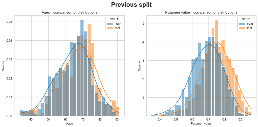
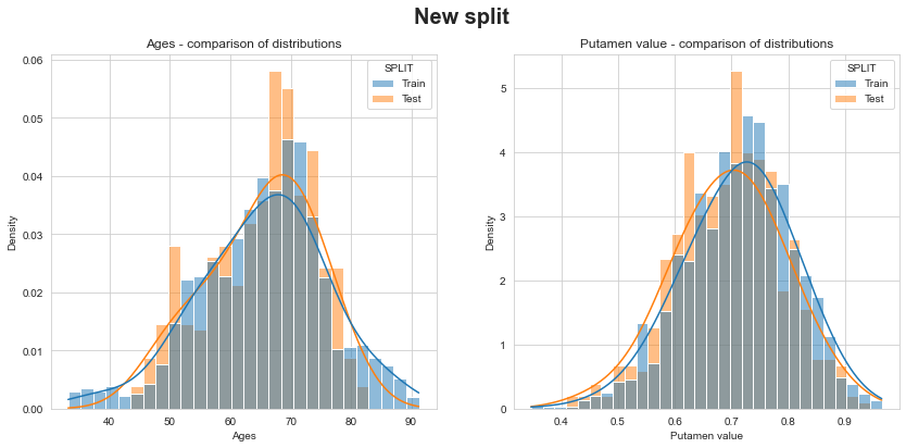
Let’s check that distributions of ages and putamen values between train & test are similar… unlike previous split!

💬 Question 49 💬 Check consistence of new train/test split and compare to previous split

df_new_split = pd.concat({
    'Train': s_train,
    'Test': s_test.droplevel(-1)
}, names=['SPLIT'])

for which_split, df_split in {'Previous split': df, 'New split': df_new_split}.items():
    fig, axs = plt.subplots(1, 2, figsize=(14,6))
    fig.suptitle(which_split, fontsize=20, fontweight='bold')
    
    for (var, title), ax in zip({'TIME': 'Ages', 'PUTAMEN': 'Putamen value'}.items(), axs):

        sns.histplot(data=df_split.reset_index(), x=var, 
                     hue='SPLIT', stat='density', common_norm=False, 
                     kde=True, kde_kws=dict(bw_adjust=2.), ax=ax)
        ax.set_title(f'{title} - comparison of distributions')
        ax.set_xlabel(title)

    plt.show()

#sns.scatterplot(data=s_train.reset_index(), 
#                x='TIME', y='PUTAMEN', alpha=.5, s=60)
#sns.scatterplot(data=s_test.reset_index(), 
#                x='TIME', y='PUTAMEN', alpha=.5, s=60)

💬 Question 50 💬 Double check number of individuals and visits in each split of our dataset

# Some descriptive stats on number of visits in test set (present part)

pd.options.display.float_format = '{:.1f}'.format

print('Visits in each split')
print({'Train': len(s_train), 
       'All test': len(s_test), 
       'Test - known part': len(s_test_present),
       'Test - to predict part': len(s_test_future)
      })
print()

print('Visits per individual in each split')
pd.concat({
    'Calibration': s_train.groupby('ID').size().describe(percentiles=[]), # min: 3 tpts known
    'Personalization': s_test_present.groupby('ID').size().describe(percentiles=[]), # min: 1 tpt known
    'Prediction': s_test_future.groupby('ID').size().describe(percentiles=[]), # min: 2 tpts to predict
}).unstack(0).rename({'count':'nb of individuals'}, axis=0)

Visits in each split
{'Train': 1499, 'All test': 498, 'Test - known part': 398, 'Test - to predict part': 100}

Visits per individual in each split

	Calibration	Personalization	Prediction
nb of individuals	150.0	50.0	50.0
mean	10.0	8.0	2.0
std	2.5	2.5	0.0
min	3.0	1.0	2.0
50%	10.0	8.0	2.0
max	18.0	13.0	2.0

💬 Question 51 💬 Write a all-in-one personalization & prediction function thanks to Leaspy api

def personalize_model(leaspy_model, settings_perso):
    """
    all-in-one function that:
    1. takes a calibrated leaspy model, 
    2. personalizes it with different splits of data
    3. and estimates prediction errors compared to real data (including the hidden parts)
    """

    ips_test = {}
    rmse_test = {}

    # personalize on train part just to have a comparison (baseline)
    ips_test['train'], rmse_test['train'] = leaspy_model.personalize(data_train, settings_perso, 
                                                                     return_noise=True)
    print(f'RMSE on train: {100*rmse_test["train"]:.2f}%')

    # personalize using different test parts
    for test_part, data_test_part in data_test.items():
        ips_test[test_part], rmse_test[test_part] = leaspy_model.personalize(data_test_part, settings_perso, 
                                                                             return_noise=True)
        print(f'RMSE on test {test_part}: {100*rmse_test[test_part]:.2f}%')
    
    # reconstruct using different personalizations made
    s_train_ix = s_train.assign(PART='train').set_index('PART',append=True).index # with fake part added
    
    all_recons_df = pd.concat({
        test_part: leaspy_model.estimate(s_test.index if test_part != 'train' else s_train_ix, 
                                         ips_test_part)
        for test_part, ips_test_part in ips_test.items()
    }, names=['PERSO_ON']).reorder_levels([1,2,3,0])

    # compute prediction errors made
    true_vals_same_ix = all_recons_df[[]].join(df.droplevel(-1).iloc[:,0])
    pred_errs = all_recons_df - true_vals_same_ix
    
    # return everything that could be needed
    return pred_errs, all_recons_df, ips_test, rmse_test

💬 Question 52 💬 Calibrate, personalize & predict with LMM, univariate linear & univariate logistic thanks to Leaspy

## Leaspy LMM (using integrated exact personalization formula)

leaspy_lmm = Leaspy('lme')
settings_fit = AlgorithmSettings('lme_fit', 
                                 with_random_slope_age=True,
                                 force_independent_random_effects=True, # orthogonal rand. eff.
                                 seed=0)

# ------- Compute population parameters on train data ------- 
# (fixed effects, noise level and var-covar of random effects)
leaspy_lmm.fit(data_train, settings_fit)

# ------- Compute individual parameters (random effects) on different splits -------
pred_errs_lmm, all_recons_df_lmm, _, _  = personalize_model(leaspy_lmm, AlgorithmSettings('lme_personalize'))

 ==> Setting seed to 0
The standard deviation of the noise at the end of the calibration is: 0.0218
RMSE on train: 1.98%
RMSE on test all: 1.91%
RMSE on test present: 1.88%
RMSE on test future: 1.61%

## Leaspy univariate linear
leaspy_lin = Leaspy('univariate_linear')
settings_fit = AlgorithmSettings('mcmc_saem', n_iter=8000, progress_bar=True, seed=0)
settings_perso = AlgorithmSettings('scipy_minimize', progress_bar=True, use_jacobian=True)

# ------- Compute population parameters on train data ------- 
leaspy_lin.fit(data_train, settings_fit)

# ------- Compute individual parameters on different splits -------
pred_errs_lin, all_recons_df_lin, _, _  = personalize_model(leaspy_lin, settings_perso)

 ==> Setting seed to 0
|##################################################|   8000/8000 iterations
The standard deviation of the noise at the end of the calibration is:
0.0216

Calibration took: 22s
|##################################################|   150/150 subjects
The standard deviation of the noise at the end of the personalization is:
0.0194

Personalization scipy_minimize took: 4s
RMSE on train: 1.94%
|##################################################|   50/50 subjects
The standard deviation of the noise at the end of the personalization is:
0.0186

Personalization scipy_minimize took: 1s
RMSE on test all: 1.86%
|##################################################|   50/50 subjects
The standard deviation of the noise at the end of the personalization is:
0.0178

Personalization scipy_minimize took: 2s
RMSE on test present: 1.78%
|##################################################|   50/50 subjects
The standard deviation of the noise at the end of the personalization is:
0.0162

Personalization scipy_minimize took: 1s
RMSE on test future: 1.62%

## Leaspy univariate logistic
leaspy_log = Leaspy('univariate_logistic')

# Calibrate
leaspy_log.fit(data_train, settings_fit)

# Personalize
pred_errs_log, all_recons_df_log, _, _  = personalize_model(leaspy_log, settings_perso)

 ==> Setting seed to 0
|##################################################|   8000/8000 iterations
The standard deviation of the noise at the end of the calibration is:
0.0215

Calibration took: 30s
|##################################################|   150/150 subjects
The standard deviation of the noise at the end of the personalization is:
0.0194

Personalization scipy_minimize took: 5s
RMSE on train: 1.94%
|##################################################|   50/50 subjects
The standard deviation of the noise at the end of the personalization is:
0.0184

Personalization scipy_minimize took: 1s
RMSE on test all: 1.84%
|##################################################|   50/50 subjects
The standard deviation of the noise at the end of the personalization is:
0.0177

Personalization scipy_minimize took: 2s
RMSE on test present: 1.77%
|##################################################|   50/50 subjects
The standard deviation of the noise at the end of the personalization is:
0.0162

Personalization scipy_minimize took: 1s
RMSE on test future: 1.62%

💬 Question 53 💬 Display RMSE on all splits of data depending on models & part where models were personalized on

# reconstruct using different personalizations made
pd.options.display.float_format = '{:.5f}'.format

all_pred_errs = pd.concat({
    'lmm': pred_errs_lmm,
    'leaspy_linear': pred_errs_lin,
    'leaspy_logistic': pred_errs_log,
}, names=['MODEL'])

print('RMSE by:\n- model\n- part of data for personalization\n- part of data for reconstruction\n')

rmses_by_perso_split = (all_pred_errs**2).groupby(['MODEL','PERSO_ON','PART']).mean() ** .5
rmses_by_perso_split.unstack('MODEL').droplevel(0, axis=1).sort_index(ascending=[True,False]).rename_axis(index={'PART':'RECONS_ON'})

RMSE by:
- model
- part of data for personalization
- part of data for reconstruction

	MODEL	lmm	leaspy_linear	leaspy_logistic
PERSO_ON	RECONS_ON
all	present	0.01897	0.01841	0.01821
all	future	0.01944	0.01910	0.01913
future	present	0.04730	0.04808	0.04923
future	future	0.01609	0.01618	0.01616
present	present	0.01880	0.01776	0.01775
present	future	0.02692	0.02666	0.02538
train	train	0.01979	0.01942	0.01941

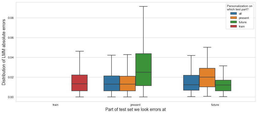
💬 Question 54 💬 Plot distributions of absolute errors

def plot_dist_errs(pred_errs, model_name, grouping_reverse=False):
    plt.figure(figsize=(14,6))
    plt.grid(True,axis='both',zorder=-1)

    plot_opts = dict(
        x='PART', order=['train','present','future'],
        hue='PERSO_ON', hue_order=['all','present','future','train'],
    )
    x_lbl = 'Part of test set we look errors at'
    legend_lbl = 'Personalization on\nwhich test part?'
    
    if grouping_reverse:
        plot_opts = dict(
            hue='PART', hue_order=['train','present','future'],
            x='PERSO_ON', order=['all','present','future','train'],
        )
        x_lbl, legend_lbl = legend_lbl, x_lbl # swap
    
    sns.boxplot(data=pred_errs.abs().reset_index(),
                y='PUTAMEN', **plot_opts, showfliers=False)

    plt.ylabel(f'Distribution of {model_name} absolute errors', fontsize=14)
    
    plt.xlabel(x_lbl, fontsize=14)
    plt.legend().set_title(legend_lbl)

plot_dist_errs(pred_errs_lmm, 'LMM')
plot_dist_errs(pred_errs_lmm, 'LMM', True)

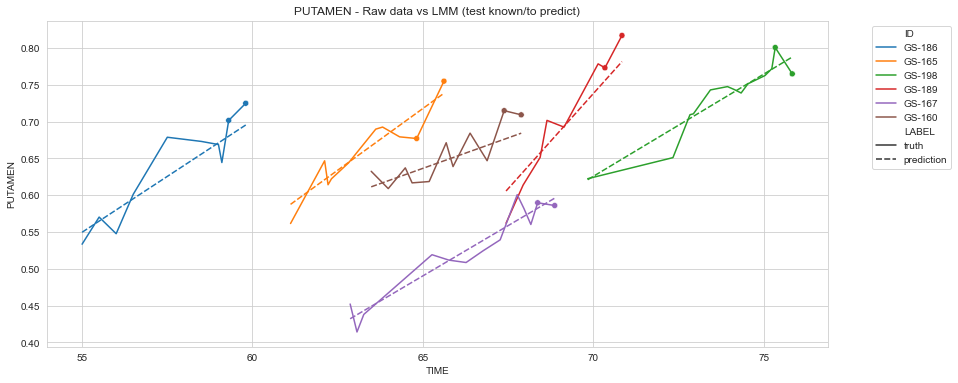
💬 Question 55 💬 Plot some individual trajectories with their associated predicted trajectories

idx_list = np.random.RandomState(5).choice(s_test.index.unique('ID'), 6).tolist()

def plot_recons(all_recons_df, model_name):

    recontruction_and_raw_data = pd.concat({'truth': s_test, 
                                            'prediction': all_recons_df.xs('present', level='PERSO_ON')
                                           }, names=['LABEL']).swaplevel(0,1).sort_index()

    plt.figure(figsize=(14,6))

    sns.lineplot(data=recontruction_and_raw_data.loc[idx_list].reset_index(), 
                 x='TIME', y='PUTAMEN', hue='ID', style='LABEL', style_order=['truth','prediction'])

    sns.scatterplot(data=s_test_future.loc[idx_list].reset_index(),  
                    x='TIME', y='PUTAMEN', hue='ID', legend=None)

    plt.legend(bbox_to_anchor=(1.05, 1), loc='upper left')

    title = f'PUTAMEN - Raw data vs {model_name} (test known/to predict)'
    plt.title(title)
    plt.grid(True)
    plt.show()

plot_recons(all_recons_df_lmm, 'LMM')
#plot_recons(all_recons_df_lin, 'Leaspy linear (univ.)')
#plot_recons(all_recons_df_log, 'Leaspy logistic (univ.)')

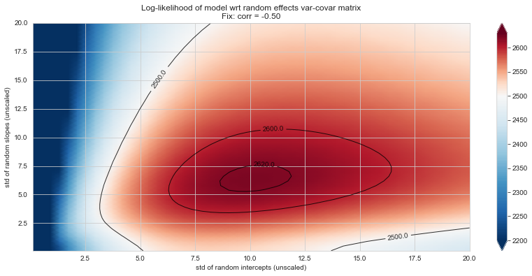
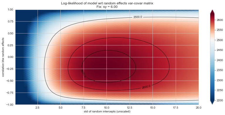
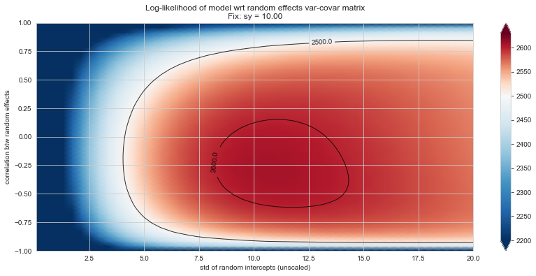
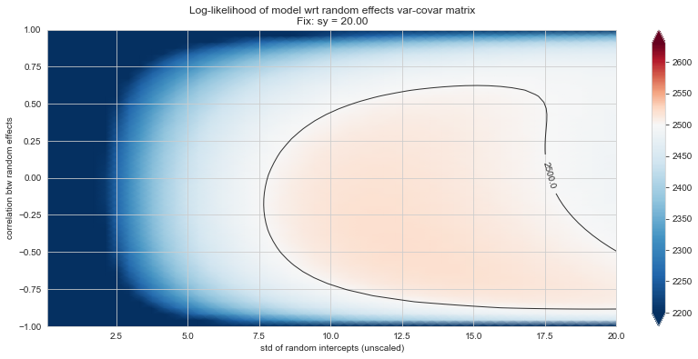
Bonus: have a look at the LMM log-likelihood landscape¶

import statsmodels.formula.api as smf
from tqdm import tqdm

import site
site.addsitedir('./utils')

from loglikelihood_landspace_lmm import plt_ll_landscape, plt_ll_landscape_

# new model (TIME_norm)
lmm_model = smf.mixedlm(formula="PUTAMEN ~ 1 + TIME_NORMALIZED", 
                        data=df.xs('train',level='SPLIT').reset_index(), 
                        groups="ID", re_formula="~ 1 + TIME_NORMALIZED")

lmm_model.cov_pen = None

view = dict(
    vmin=2200,
    vmid=2500, 
    vmax=2630, 
    levels=[2500, 2600, 2620]
)

Rs = {} # placeholder for results

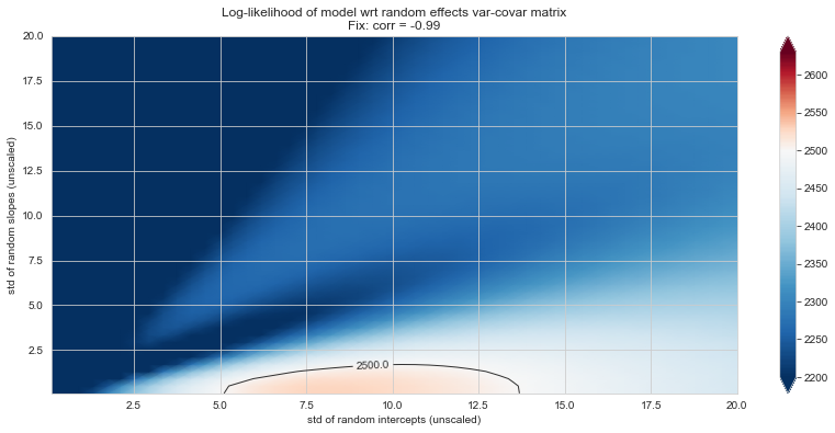
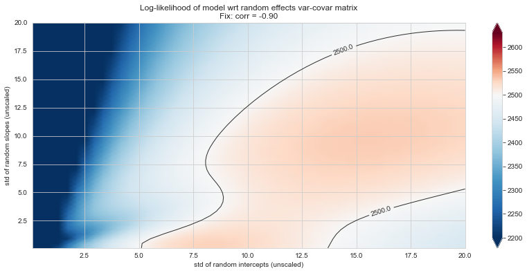
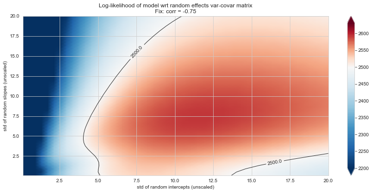
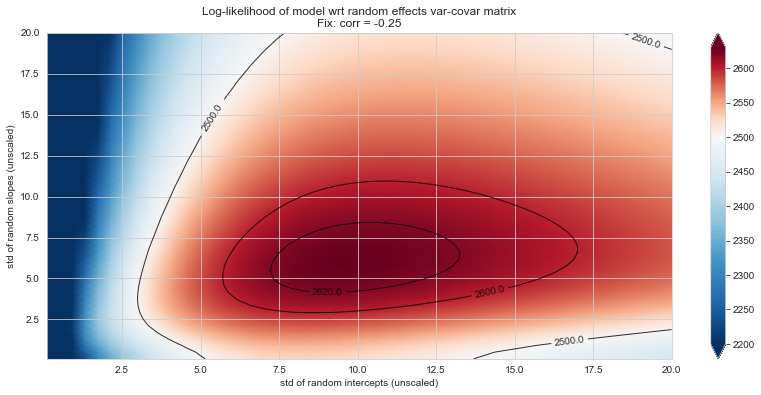
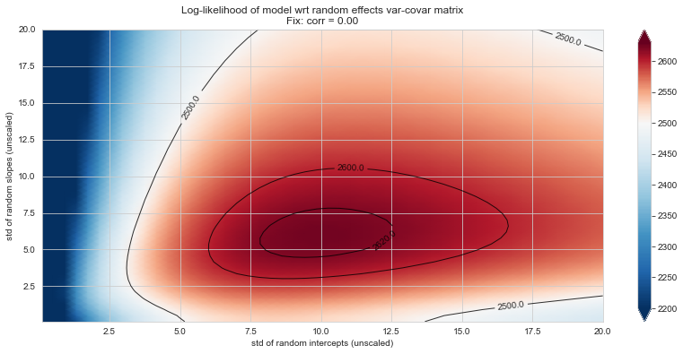
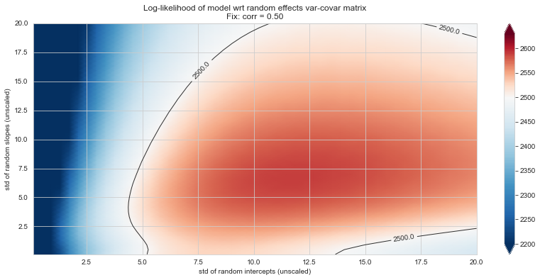
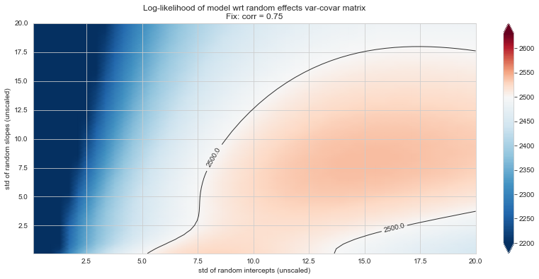
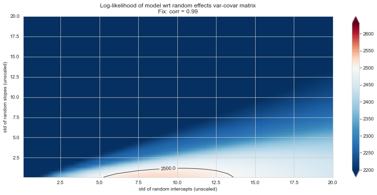
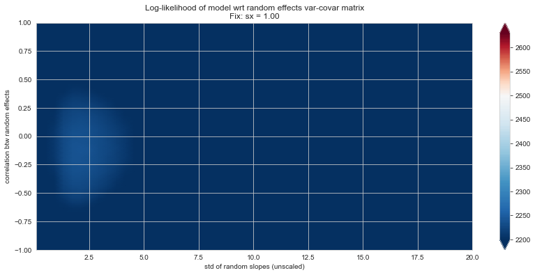
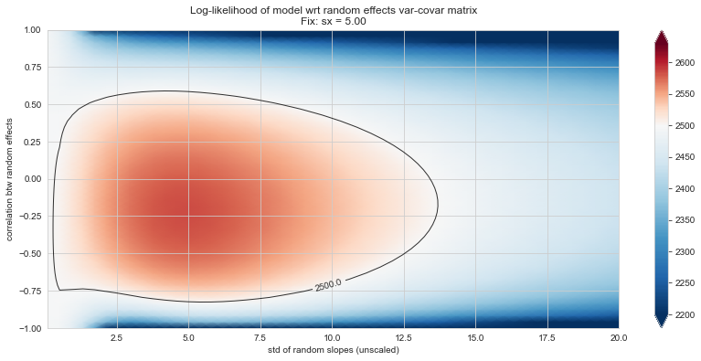
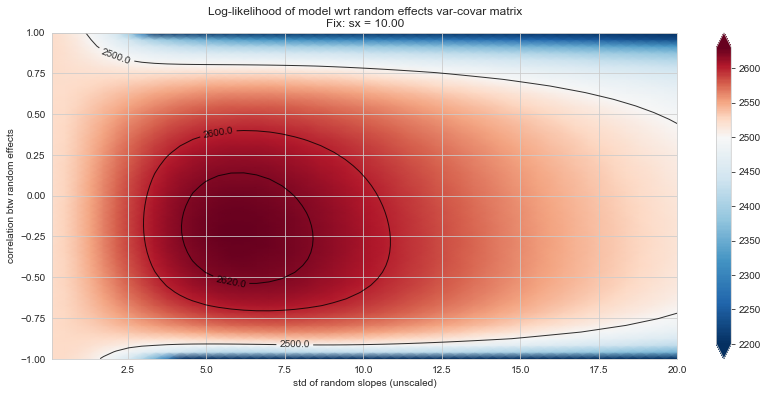
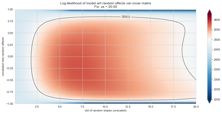
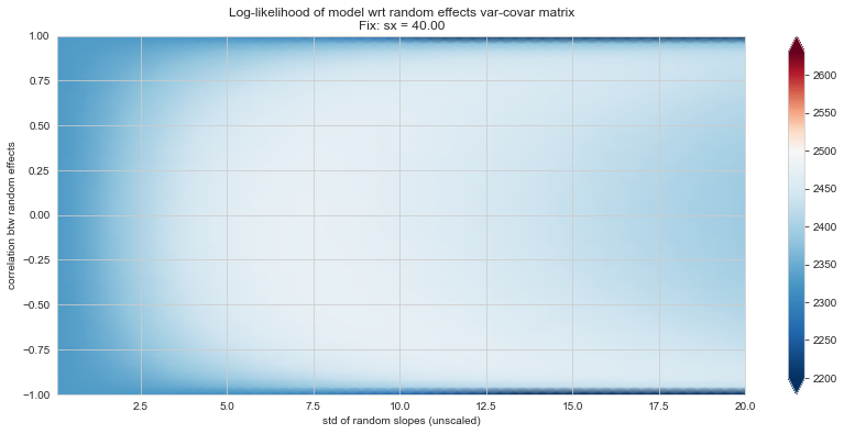
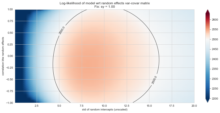
💬 Question 56 💬 Plot log-likelihood landscapes for LMM model, depending on variance-covariance matrix of random effects

for fix_k, fix_v in tqdm([
    # corr fixed
    ('corr', -.99),
    ('corr', -.9),
    ('corr', -.75),
    ('corr', -.5),
    ('corr', -.25), # ~best
    ('corr', 0),
    ('corr', .5),
    ('corr', .75),
    ('corr', .99),
    # sx fixed
    ('sx', 1.),
    ('sx', 5),
    ('sx', 10), # ~best
    ('sx', 20),
    ('sx', 40),
    # sy fixed
    ('sy', 1),
    ('sy', 6), # ~best
    ('sy', 10),
    ('sy', 20),
]):
    if (fix_k, fix_v) in Rs:
        plt_ll_landscape_(Rs[(fix_k, fix_v)], **view)
    else:
        Rs[(fix_k, fix_v)] = plt_ll_landscape(lmm_model, N=50, **{fix_k: fix_v}, **view)

  0%|          | 0/18 [00:00<?, ?it/s]

  6%|▌         | 1/18 [01:23<23:39, 83.51s/it]

 11%|█         | 2/18 [02:58<24:06, 90.39s/it]

 17%|█▋        | 3/18 [04:43<24:16, 97.10s/it]

 22%|██▏       | 4/18 [06:01<20:53, 89.53s/it]

 28%|██▊       | 5/18 [07:27<19:04, 88.05s/it]

 33%|███▎      | 6/18 [08:53<17:31, 87.61s/it]

 39%|███▉      | 7/18 [10:06<15:08, 82.59s/it]

 44%|████▍     | 8/18 [11:19<13:17, 79.72s/it]

 50%|█████     | 9/18 [12:31<11:35, 77.33s/it]/Users/etienne.maheux/Documents/repos/disease-course-mapping-solutions/TP1_LMM/utils/loglikelihood_landspace_lmm.py:130: UserWarning: No contour levels were found within the data range.
  colors='black', alpha=.8, linewidths=1)

 56%|█████▌    | 10/18 [13:44<10:07, 75.94s/it]

 61%|██████    | 11/18 [14:58<08:46, 75.22s/it]

 67%|██████▋   | 12/18 [16:11<07:27, 74.57s/it]

 72%|███████▏  | 13/18 [17:24<06:10, 74.09s/it]

 78%|███████▊  | 14/18 [18:38<04:56, 74.21s/it]

 83%|████████▎ | 15/18 [19:56<03:45, 75.18s/it]

 89%|████████▉ | 16/18 [21:14<02:32, 76.14s/it]

 94%|█████████▍| 17/18 [22:27<01:15, 75.09s/it]

100%|██████████| 18/18 [23:52<00:00, 79.58s/it]

Disease Progression Modelling

Linear Mixed-effects Models¶

Objectives :¶

The set-up¶

Part I: The data¶

Part II: Linear Regression¶

Part III: The longitudinal aspect¶

PART IV: Indivual Linear Regressions¶

Part V : Linear Mixed effects Model with statsmodels¶

Run a LMM with statsmodels¶

PART VI: A taste of the future - Linear mixed-effect model with Leaspy¶

PART VII: A taste of the future - Non-linear mixed-effect model with Leaspy¶

For the fast-running Zebras: all-in-one with a more realistic split of data¶

Bonus: have a look at the LMM log-likelihood landscape¶

Part V : Linear Mixed effects Model with `statsmodels`¶

Run a LMM with `statsmodels`¶