First steps with Leaspy#
Welcome for the second practical session of the day!
Objectives :#
Learn to use Leaspy methods
The set-up#
As before, if you have followed the installation details carefully, you should
be running this notebook in the
leaspy_tutorialvirtual environmenthaving all the needed packages already installed
💬 Question 1 💬 Run the following command lines
import os, sys
from scipy import stats
import numpy as np
import pandas as pd
import matplotlib.pyplot as plt

# import main classes from Leaspy package
sys.path.append('/Users/igor.koval/Documents/work/leaspy/')
from leaspy import Leaspy, Data, AlgorithmSettings, IndividualParameters#, __watermark__

# Watermark trace with all packages versions
#print("\n".join([f'{pkg}: {pkg_version}' for pkg, pkg_version in __watermark__.items()]))
Part I: Data#
ℹ️ Information ℹ️ Data that can be used as a leaspy input should have the following format.
This result in multiple rows per subject. The input format MUST follow the following rules:
A column named
ID: corresponds to the subject indicesA columns named
TIME: corresponds to the subject’s age at the corresponding visitOne column per feature
Each row is a visit, therefore the concatenation of the subject ID, the patient age at which the corresponding visit occured, and then the feature values
Concerning the features’ values, as we are using a logistic model, they MUST:
Be between 0 and 1
In average increase with time for each subject (normal states correspond to values near 0 and pathological states to values near 1)
Moreover, to calibrate the progression model, we highly recommend to keep subjects that have been seen at least two times. You probably noticed that there are NaN: do not worry, Leaspy can handle them ;)
💬 Question 2 💬 Run the following lines to load the data.
data_path = os.path.join(os.getcwd(), 'data', 'TP2_leaspy_beginner')
df = pd.read_csv(os.path.join(data_path, 'simulated_data-corrected.csv'))
df = df.set_index(["ID","TIME"])
df.head()
| MDS1_total | MDS2_total | MDS3_off_total | SCOPA_total | MOCA_total | REM_total | PUTAMEN_R | PUTAMEN_L | CAUDATE_R | CAUDATE_L | PUTAMEN | ||
|---|---|---|---|---|---|---|---|---|---|---|---|---|
| ID | TIME | |||||||||||
| GS-001 | 71.354607 | 0.112301 | 0.122472 | 0.171078 | 0.160001 | 0.275257 | 0.492485 | 0.780210 | 0.676774 | 0.622611 | 0.494641 | 0.728492 |
| 71.554604 | 0.140880 | 0.109504 | 0.118693 | 0.135852 | 0.380934 | 0.577203 | 0.751444 | 0.719796 | 0.618434 | 0.530978 | 0.735620 | |
| 72.054604 | 0.225499 | 0.270502 | 0.061310 | 0.211134 | 0.351172 | 0.835828 | 0.823315 | 0.691504 | 0.717099 | 0.576978 | 0.757409 | |
| 73.054604 | 0.132519 | 0.253548 | 0.258786 | 0.245323 | 0.377842 | 0.566496 | 0.813593 | 0.787914 | 0.770048 | 0.709486 | 0.800754 | |
| 73.554604 | 0.278923 | 0.321920 | 0.143350 | 0.223102 | 0.292768 | 0.741811 | 0.888792 | 0.852720 | 0.797368 | 0.715465 | 0.870756 |
💬 Question 3 💬 Does the data set seem to have the good format?
Your answer: …
💬 Question 4 💬 How many patients are there in the dataset?
# To complete
# –––––––––––––––– #
# –––– Answer –––– #
# –––––––––––––––– #

n_subjects = df.index.get_level_values('ID').unique().shape[0]
print(f'{n_subjects} subjects in the dataset.')
200 subjects in the dataset.
💬 Question 5 💬 Create a training test that contains the first 160 patients and a testing set the rest. Each set will only contain the following features:
MDS1_total
MDS2_total
MDS3_off_total
Help : Be careful, one patient is not one line …
# To complete

df_train = ######################
df_test = ######################
# –––––––––––––––– #
# –––– Answer –––– #
# –––––––––––––––– #

df_train = df.loc[:'GS-160'][["MDS1_total", "MDS2_total", "MDS3_off_total"]]
df_test = df.loc['GS-161':][["MDS1_total", "MDS2_total", "MDS3_off_total"]]
Leaspy’s Data container#
ℹ️ Information ℹ️ Leaspy comes with its own data containers. The one used in a daily basis is Data. You can load your data from a csv with it Data.from_csv_file or from a DataFrame Data.from_dataframe.
💬 Question 6 💬 Run the following lines to convert DataFrame into Data object.
data_train = Data.from_dataframe(df_train)
data_test = Data.from_dataframe(df_test)
Part II : Instantiate a Leaspy object#
ℹ️ Information ℹ️ Before creating a leaspy object, you need to choose the type of progression shape you want to give to your data. The available models are the following:
linear
logistic
with the possibility to enforce a parallelism between the features. Parallelism imposes that all the features have the same average pace of progression.
Once that is done, you just have to call Leaspy('model_name'). The dedicated names are :
univariate_linearlinearunivariate_logisticlogisticlogistic_parallellme_modelconstant_model
💬 Question 7 💬 We choose a logistic model. Run the following line to instantiate the leaspy object.
leaspy = Leaspy("logistic", source_dimension=2)
ℹ️ Information ℹ️ Leaspy object contains all the main methods provided by the software. With this object, you can:
calibrate a model
personalize a model to individual data (basically you infer the random effects with a gradient descent)
estimate the features values of subjects at given ages based on your calibrated model and their individual parameters
simulate synthetic subjects base on your calibrated model, a collection of individual parameters and data
load and save a model
💬 Question 8 💬 Check it out by running the following line
? Leaspy
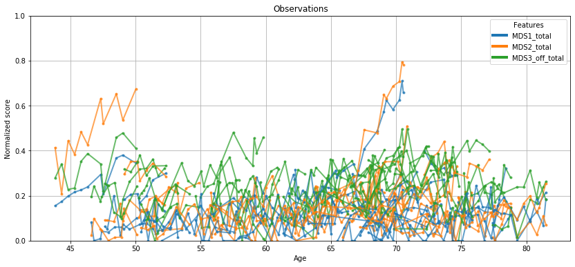
💬 Question 9 💬 This Leaspy object comes with an handy attribute for vizualization. Let’s have a look on the data that will be used to calibrate our model
leaspy.model.dimension
ax = leaspy.plotting.patient_observations(data_train, alpha=.7, figsize=(14, 6))
ax.set_ylim(0,.8)
ax.grid()
plt.show()
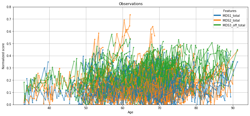
Well… not so engaging, right? Let’s see what Leaspy can do for you.
Part III : Choose your algorithms#
ℹ️ Information ℹ️ Once you choosed your model, you need to choose an algorithm to calibrate it.
To run any algorithm, you need to specify the settings of the related algorithm thanks to the AlgorithmSettings object. To ease Leaspy’s usage for new users, we specified default values for each algorithm. Therefore, the name of the algorithm used is enough to run it. The one you need to fit your progression model is mcmc_saem, which stands for Markov chain Monte Carlo - Stochastic Approximation of Expectation Maximization.
💬 Question 10 💬 Run the following line to instanciate a AlgorithmSettings object.
algo_settings = AlgorithmSettings('mcmc_saem',
                                  n_iter=2000,           # n_iter defines the number of iterations
                                  loss='MSE_diag_noise', # estimate the residual noise scaling per feature
                                  progress_bar=True)     # To display a nice progression bar during calibration
ℹ️ Information ℹ️ You can specify many more settings that are left by default for now. You can also save and load an AlgorithmSettings object in a json file.
💬 Question 11 💬 Run the following line to get more informations.
? AlgorithmSettings
ℹ️ Information ℹ️ It is often usefull, even if it is optional to store the different logs of the model during the iterations. You can use the following method with the path of the folder where the logs will be stored.
💬 Question 12 💬 Run the following lines.
algo_settings.set_logs(
    path='logs',          # Creates a logs file ; if existing, ask if rewrite it
    plot_periodicity=50,  # Saves the values to display in pdf every 50 iterations
    save_periodicity=10,  # Saves the values in csv files every 10 iterations
    console_print_periodicity=None,  # If = N, it display logs in the console/terminal every N iterations
    overwrite_logs_folder=True       # Default behaviour raise an error if the folder already exists.
)
...overwrite logs folder...
Part IV : Fit your model#
💬 Question 13 💬 Run the following lines to fit the model.
leaspy.fit(data_train, algorithm_settings=algo_settings)
|##################################################|   2000/2000 iterations
The standard deviation of the noise at the end of the calibration is:
MDS1_total: 0.0512
MDS2_total: 0.0544
MDS3_off_total: 0.0649

Calibration took: 1min 22s
ℹ️ Information ℹ️ This might take several minutes, so let’s discuss about the keyword argument source_dimension. This parameters depend on the number of variable you want the model to learn: it can go from 1 to the number of variables. If it is not set by the user the default value is \(\sqrt{N_{features}}\) as it has been shown empirically to give good results. You will learn more about the mathematical formulation of the model below (part V).
ℹ️ Information ℹ️ Before assuming that the model is estimated, you have to check that the convergence went well. For that, you can look the at the convergence during the iterations. To do so, you can explore the logs folder (in the same folder than this jupyter notebook) that shows the model convergence during the iterations. The first thing to look at is probably the plots/convergence_1.pdf and plots/convergence_2.pdf files : a run has had enough iterations to converge if the last 20 or even 30% of the iterations were stable for all the parameters. If not, you should provably re-run it with more iterations.
from IPython.display import IFrame
IFrame('./logs/plots/convergence_1.pdf', width=990, height=670)
💬 Question 14 💬 Check out the parameters of the model that are stored here
leaspy.model.parameters
{'g': tensor([1.9860, 1.8967, 1.2987]),
 'v0': tensor([-4.7647, -4.5189, -4.6165]),
 'betas': tensor([[ 0.0230,  0.0497],
         [-0.0321,  0.0040]]),
 'tau_mean': tensor(65.0794),
 'tau_std': tensor(10.3418),
 'xi_mean': tensor(0.),
 'xi_std': tensor(0.5935),
 'sources_mean': tensor(0.),
 'sources_std': tensor(1.),
 'noise_std': tensor([0.0512, 0.0544, 0.0649])}
ℹ️ Information ℹ️ Parameters are probably not straightfoward for now. The most important one is probably noise_std. It corresponds to the standard deviation of the Gaussian errors (one per feature). The smallest, the better - up to the lower bound which is the intrinsic noise in the data. Note that usually, cognitive measurements have an intrinsic error (computed on test-retest exams) between 5% and 10%.
💬 Question 15 💬 Let’s display noise_std
noise = leaspy.model.parameters['noise_std']
features = leaspy.model.features

print('Standard deviation of the residual noise for the feature:')
for n, f in zip(noise, features):
    print(f'- {f}: {n*100:.2f}%')
Standard deviation of the residual noise for the feature:
- MDS1_total: 5.12%
- MDS2_total: 5.44%
- MDS3_off_total: 6.49%
💬 Question 16 💬 Save the model with the command below
leaspy.save(os.path.join(data_path, "model_parameters.json"), indent=2)
💬 Question 17 💬 Load the model with the command below
leaspy = Leaspy.load(os.path.join(data_path, 'model_parameters.json'))
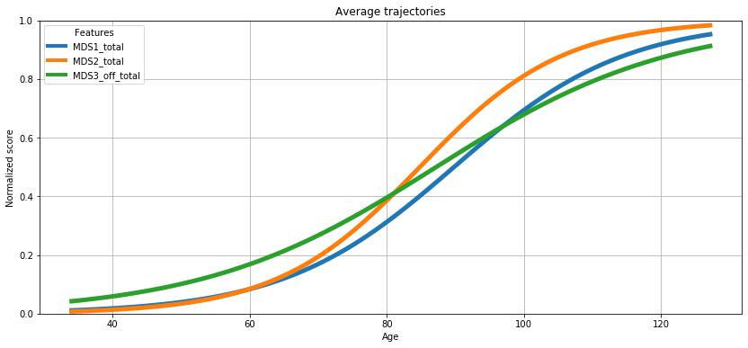
ℹ️ Information ℹ️ Now that we have sufficient evidence that the model has converged, let’s output what the average progression looks like!
First, let’s detail a bit what we are going to represent. We are going to display a trajectory: it corresponds to the temporal progression of the biomarkers. There is not only one trajectory for a cohort, as each subject has his or her own specific trajectory, meaning his or her disease progression. Each of these individual trajectories rely on individual parameters that are subject-specific. We will see those individual parameters a bit later, do not worry. For now, let’s stick to the average trajectory.
So what does the average trajectory corresponds to? The average trajectory correspond to a virtual patient whose individual parameters are the average individual parameters. And these averages are already estimated during the calibration.
💬 Question 18 💬 Let’s plot the average trajectory
ax = leaspy.plotting.average_trajectory(alpha=1, figsize=(14,6))
ax.grid()
plt.show()
Part V : Personalize the model to individual data#
ℹ️ Information ℹ️ The personalization procedure allows to estimate the individual parameters that allows to modify the average progression to individual observations. The variations from the average trajectory to the individual one are encoded within three individual parameters :
\(\alpha_i = \exp(\xi_i)\) : the acceleration factor, that modulates the speed of progression : \(\alpha_i > 1\) means faster, \(\alpha_i < 1\) means slower than the average progression
\(\tau_i\) : the time shift which delays the progression in a given number of years. It has to be compared to
tau_mean\( = \bar{\tau} \) which is in the model parameters above. In fact, \( \tau_i \sim \mathcal{N}( \bar{\tau}, \sigma_{\tau}^2)\) , so \(\tau_i > \bar{\tau}\) means that the patient has a disease that starts later than average, while \(\tau_i < \bar{\tau}\) means that the patient has a disease that starts earlier than average\(w_i = (w_1, ..., w_N)\) (\(N\) being the number of features) : the space-shift which might, for a given individual, change the ordering of the conversion of the different features, compared to the mean trajectory.
In a nutshell, the \(k\)-th feature at the \(j\)-th visit of subject \(i\), which occurs at time \(t_{ij}\) writes:
With:
\(\theta\) being the population parameters, infered during calibration of the model,
\(f_\nu\) a parametric family of trajectories depending of model type,
\(\epsilon_{ijk}\) an independent normally distributed error term.
This writing is not exactly correct but helps understand the role of each individual parameters.
[ Advanced ] Remember the sources, or the source_dimension? Well, \(w_i\) is not estimated directly, but rather thanks to a Independant Component Analysis, such that \(w_i = A s_i\) where \(s_i\) is of dimension \(N_s\) = source_dimension. See associated papers for further details.
Now, let’s estimate these individual parameters. The procedure relies on the scipy_minimize algorithm (gradient descent) that you have to define (or to load from an appropriate json file) :
💬 Question 19 💬 First set the parameters
settings_personalization = AlgorithmSettings('scipy_minimize', progress_bar=True, use_jacobian=True)
💬 Question 20 💬 Then use the second most important function of leaspy : leaspy.personalize. It estimates the individual parameters for the data you provide:
?leaspy.personalize
ip = leaspy.personalize(data_test, settings_personalization)
|########################################|   40/40 subjects
The standard deviation of the noise at the end of the personalization is:
MDS1_total: 0.0466
MDS2_total: 0.0492
MDS3_off_total: 0.0582

Personalization scipy_minimize took: 2s
ℹ️ Information ℹ️ Note here that you can personalize your model on patients that have only one visit! And you don’t have to use the same data as previously. It is especially useful, and important, in order to validate your model!
💬 Question 20b 💬 Once the personalization is done, check the different functions that the IndividualParameters provides (you can save and load them, transform them to dataframes, etc) :
?ip
💬 Question 21 💬 Plot the test data, but with reparametrized ages instead of real ages
# Plot the test data with individually reparametrized ages
ax = leaspy.plotting.patient_observations_reparametrized(data_test, ip,
                                                         alpha=.7, linestyle='-',
                                                         #patients_idx=list(data_test.individuals.keys())[:20],
                                                         figsize=(14, 6))
ax.grid()
plt.show()
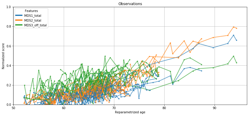
Remember the raw plotting of values during question 9? Better, no?
# Plot the test data with individually with true ages
ax = leaspy.plotting.patient_observations(data_test,
                                          alpha=.7, linestyle='-',
                                          #patients_idx=list(data_test.individuals.keys())[:4],
                                          figsize=(14, 6))
ax.grid()
plt.show()
Now, let’s see what you can do with the individual parameters.
Part VI : Impute missing values & predict individual trajectories#
ℹ️ Information ℹ️ Together with the population parameters, the individual parameters entirely defines the individual trajectory, and thus, the biomarker values at any time. So you can reconstruct the individual biomarkers at different ages.
You can reconstruct your observations at seen ages, i.e. at visits that have been used to personalize the model. There are two reasons you might want to do that:
see how well the model fitted individual data
impute missing values: as Leaspy handles missing values, it can then reconstruct them (note that this reconstruction will be noiseless)
The third very important function - after leaspy.fit and leaspy.personalize - is leaspy.estimate. Given some individual parameters and timepoints, the function estimates the values of the biomarkers at the given timepoints which derive from the individual trajectory encoded thanks to the individual parameters.
💬 Question 22 💬 Check out the documentation
?leaspy.estimate
💬 Question 23 💬 Before running leaspy.estimate, let’s first retrieve the observations of subject ‘GS-187’ in the initial dataset. Get also his/her individual parameters as shown here:
observations = df_test.loc['GS-187']
print(f'Seen ages: {observations.index.values}')
print("Individual Parameters : ", ip['GS-187'])
Seen ages: [61.34811783 62.34811783 63.84811783 64.34812164 67.84812164 68.34812164
 69.34812164 69.84812164 70.84812164 71.34812164 71.84812164 72.34812164
 72.84812164 73.34812164]
Individual Parameters :  {'xi': 8.263221388915554e-05, 'tau': 70.71927642822266, 'sources': [0.8920779228210449, -0.9051297903060913]}
ℹ️ Information ℹ️ The estimate first argument is a dictionary, so that you can estimate the trajectory of multiple individuals simultaneously (as long as the individual parameters of all your queried patients are in ip.
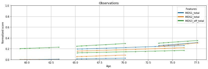
💬 Question 24 💬 Now, let’s estimate the trajectory for this patient.
timepoints = np.linspace(60, 100, 100)
reconstruction = leaspy.estimate({'GS-187': timepoints}, ip)

def plot_trajectory(timepoints, reconstruction, observations=None):

    if observations is not None:
        ages = observations.index.values

    plt.figure(figsize=(14, 6))
    plt.grid()
    plt.ylim(0, .75)
    plt.ylabel('Biomarker normalized value')
    plt.xlim(60, 100)
    plt.xlabel('Patient age')
    colors = ['#003f5c', '#7a5195', '#ef5675', '#ffa600']

    for c, name, val in zip(colors, leaspy.model.features, reconstruction.T):
        plt.plot(timepoints, val, label=name, c=c, linewidth=3)
        if observations is not None:
            plt.plot(ages, observations[name], c=c, marker='o', markersize=12)

    plt.legend()
    plt.show()

plot_trajectory(timepoints, reconstruction['GS-187'], observations)
/usr/local/Cellar/graph-tool/2.35/libexec/lib/python3.8/site-packages/matplotlib/cbook/__init__.py:1402: FutureWarning: Support for multi-dimensional indexing (e.g. `obj[:, None]`) is deprecated and will be removed in a future version.  Convert to a numpy array before indexing instead.
  x[:, None]
/usr/local/Cellar/graph-tool/2.35/libexec/lib/python3.8/site-packages/matplotlib/axes/_base.py:278: FutureWarning: Support for multi-dimensional indexing (e.g. `obj[:, None]`) is deprecated and will be removed in a future version.  Convert to a numpy array before indexing instead.
  y = y[:, np.newaxis]
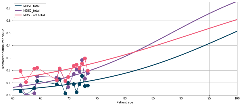
data_test.to_dataframe().set_index(['ID']).loc['GS-187']
| TIME | MDS1_total | MDS2_total | MDS3_off_total | |
|---|---|---|---|---|
| ID | ||||
| GS-187 | 61.348118 | 0.032155 | 0.079023 | 0.194349 |
| GS-187 | 62.348118 | 0.000000 | 0.000000 | 0.105951 |
| GS-187 | 63.848118 | 0.056661 | 0.015366 | 0.213064 |
| GS-187 | 64.348122 | 0.113765 | 0.151636 | 0.220763 |
| GS-187 | 67.848122 | 0.087926 | 0.142727 | 0.121259 |
| GS-187 | 68.348122 | 0.127519 | 0.208425 | 0.215517 |
| GS-187 | 69.348122 | 0.014113 | 0.116000 | 0.115312 |
| GS-187 | 69.848122 | 0.098333 | 0.067149 | 0.147486 |
| GS-187 | 70.848122 | 0.088108 | 0.168970 | 0.235806 |
| GS-187 | 71.348122 | 0.025140 | 0.206862 | 0.245327 |
| GS-187 | 71.848122 | 0.088468 | 0.193132 | 0.215797 |
| GS-187 | 72.348122 | 0.156485 | 0.281915 | 0.255358 |
| GS-187 | 72.848122 | 0.072483 | 0.134019 | 0.297301 |
| GS-187 | 73.348122 | 0.076749 | 0.177526 | 0.196283 |
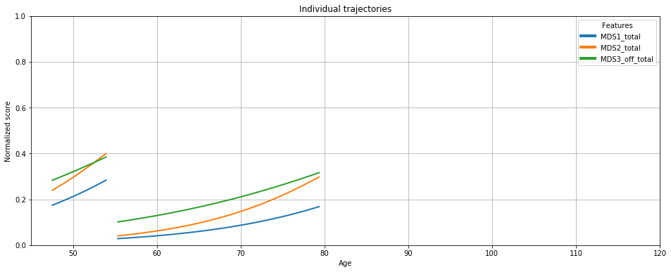
# Or with plotting object
ax = leaspy.plotting.patient_trajectories(data_test, ip,
                                          patients_idx=['GS-187','GS-180'],
                                          labels=['MDS1_total','MDS2_total', 'MDS3_off_total'],
                                          #reparametrized_ages=True, # check sources effect

                                          # plot kwargs
                                          #color=['#003f5c', '#7a5195', '#ef5675', '#ffa600'],
                                          alpha=1, linestyle='-', linewidth=2,
                                          #marker=None,
                                          markersize=8, obs_alpha=.5, #obs_ls=':',
                                          figsize=(16, 6),
                                          factor_past=.5,
                                          factor_future=5, # future extrapolation
                                          )
ax.grid()
#ax.set_ylim(0, .75)
ax.set_xlim(45, 120)
plt.show()
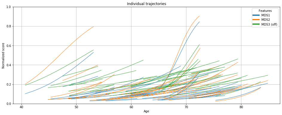
# Grasp source effects
ax = leaspy.plotting.patient_trajectories(data_test, ip,
                                          patients_idx='all',
                                          labels=['MDS1','MDS2', 'MDS3 (off)'],
                                          reparametrized_ages=True, # check sources effect

                                          # plot kwargs
                                          alpha=1, linestyle='-', linewidth=1,
                                          marker=None,
                                          figsize=(16, 6),
                                          factor_past=0,
                                          factor_future=0, # no extrapolation (future) nor past
                                          )
ax.grid()
#ax.set_ylim(0, .75)
#ax.set_xlim(45, 120)
plt.show()
Part VII : Leaspy application - Cofactor analysis#
ℹ️ Information ℹ️ Besides prediction, the individual parameters are interesting in the sense that they provide meaningful and interesting insights about the disease progression. For that reason, these individual parameters can be correlated to other cofactors. Let’s consider that you have a covariate Cofactor 1 that encodes a genetic status: 1 if a specific mutation is present, 0 otherwise.
💬 Question 25 💬 Now, let’s see if this mutation has an effect on the disease progression:
import seaborn as sns
# —— Convert individual parameters to dataframe
df_ip = ip.to_dataframe()
# —— Join the cofactors to individual parameters
cofactor = pd.read_csv(os.path.join(data_path, "cof_leaspy1.csv"), index_col=['ID'])
df_ip = df_ip.join(cofactor.replace({'MUTATION':{0: 'Non-carrier', 1: 'Carrier'}}))
_, ax = plt.subplots(1, 2, figsize=(14, 6))
# —— Plot the time shifts in carriers and non-carriers
ax[0].set_title('Time shift histogram')
sns.histplot(data=df_ip, x='tau', hue='MUTATION', bins=15, ax=ax[0], stat='count', common_norm=False, kde=True)
# —— Plot the acceleration factor in carriers and non-carriers
ax[1].set_title('Log-Acceleration factor histogram')
sns.histplot(data=df_ip, x='xi', hue='MUTATION', bins=15, ax=ax[1], stat='count', common_norm=False, kde=True)
plt.show()
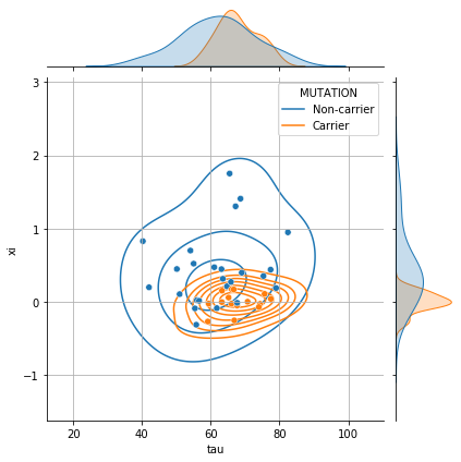
# __ Joint density (tau, xi) __
g = sns.jointplot(data=df_ip, x="tau", y="xi", hue="MUTATION", height=6)
g.plot_joint(sns.kdeplot, zorder=0, levels=8, bw_adjust=1.5)
g.ax_joint.grid();
/usr/local/Cellar/graph-tool/2.35/libexec/lib/python3.8/site-packages/matplotlib/cbook/__init__.py:1402: FutureWarning: Support for multi-dimensional indexing (e.g. `obj[:, None]`) is deprecated and will be removed in a future version.  Convert to a numpy array before indexing instead.
  x[:, None]
/usr/local/Cellar/graph-tool/2.35/libexec/lib/python3.8/site-packages/matplotlib/axes/_base.py:276: FutureWarning: Support for multi-dimensional indexing (e.g. `obj[:, None]`) is deprecated and will be removed in a future version.  Convert to a numpy array before indexing instead.
  x = x[:, np.newaxis]
/usr/local/Cellar/graph-tool/2.35/libexec/lib/python3.8/site-packages/matplotlib/axes/_base.py:278: FutureWarning: Support for multi-dimensional indexing (e.g. `obj[:, None]`) is deprecated and will be removed in a future version.  Convert to a numpy array before indexing instead.
  y = y[:, np.newaxis]
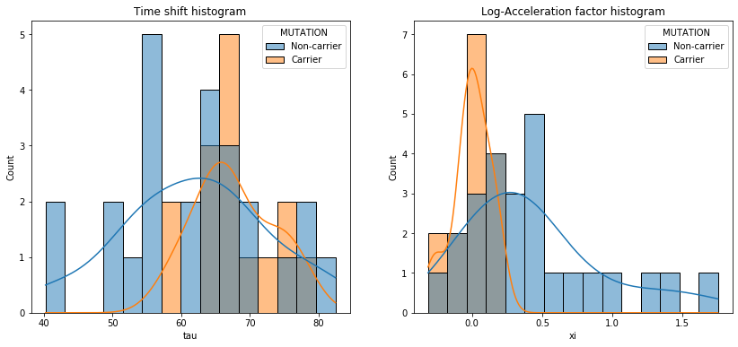
💬 Question 26 💬 Now, check your hypothesis with statistical tests
# Shortcuts of df_ip for 2 sub-populations
carriers = df_ip[df_ip['MUTATION'] == 'Carrier']
non_carriers = df_ip[df_ip['MUTATION'] == 'Non-carrier']
# —— Student t-test (under the asumption of a gaussian distribution only)
print(stats.ttest_ind(carriers['tau'], non_carriers['tau']))
print(stats.ttest_ind(carriers['xi'], non_carriers['xi']))

# —— Mann-withney t-test
print(stats.mannwhitneyu(carriers['tau'], non_carriers['tau']))
print(stats.mannwhitneyu(carriers['xi'], non_carriers['xi']))
Ttest_indResult(statistic=1.941230030309452, pvalue=0.059673501020270414)
Ttest_indResult(statistic=-3.3108067640055814, pvalue=0.0020460286770261965)
MannwhitneyuResult(statistic=120.0, pvalue=0.030617610211415968)
MannwhitneyuResult(statistic=65.0, pvalue=0.00032679719774224823)
Part VIII : Data Simulation#
ℹ️ Information ℹ️ Now that you are able to predict the evolution of a patient and use it to analyse cofactors, you might want to simulate a new one thanks to the information that you have learned. To do so you can use the last method of leaspy that we will study : simulate.
💬 Question 27 💬 Have a look to the function
?leaspy.simulate
ℹ️ Information ℹ️ To use the fuction we will first extract the individual parameters using personalize with mode_real option. The simulate function learns the joined distribution of the individual parameters and baseline age of the subjects
present in individual_parameters and data respectively to sample new patients from this joined distribution.
💬 Question 28 💬 Define the settings for the personalization and get the individual parameters
settings_ip_simulate = AlgorithmSettings('mode_real')
individual_params = leaspy.personalize(data_test, settings_ip_simulate)
The standard deviation of the noise at the end of the personalization is:
MDS1_total: 0.0469
MDS2_total: 0.0494
MDS3_off_total: 0.0583

Personalization mode_real took: 6s
💬 Question 29 💬 Define your algorithm for the simulation and simulate individuals from previously obtained individual parameters and dataset
settings_simulate = AlgorithmSettings('simulation')
simulated_data = leaspy.simulate(individual_params, data_test, settings_simulate)
💬 Question 30 💬 Access to the individual parameters of one individual that you have created
print(simulated_data.get_patient_individual_parameters("Generated_subject_001"))
{'tau': tensor([65.7623], dtype=torch.float64), 'xi': tensor([0.5340], dtype=torch.float64), 'sources': tensor([1.5067, 0.3401], dtype=torch.float64)}
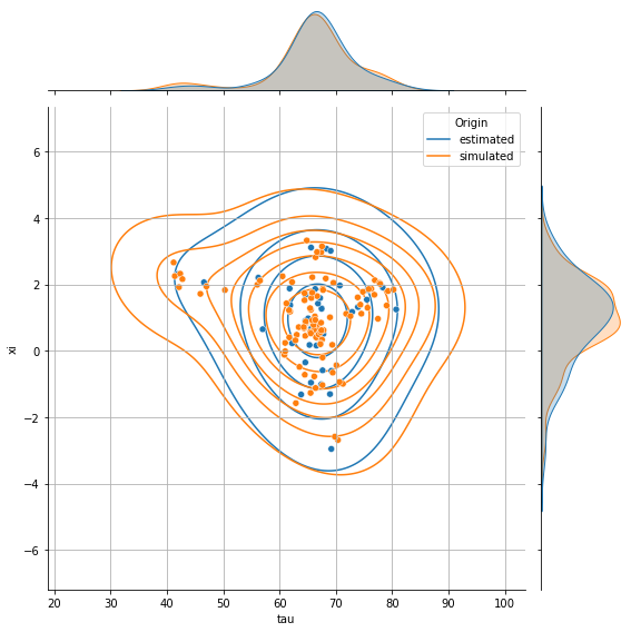
💬 Question 31 💬 Plot the joint distribution of individual parameters (tau, xi) for simulated individuals that you have created
# Create a dataframe with individual parameters from both real & simulated individuals
df_ip_both = pd.concat({
    'estimated': individual_params.to_dataframe(),
    'simulated': simulated_data.get_dataframe_individual_parameters()
}, names=['Origin'])

g = sns.jointplot(data=df_ip_both, x='tau', y='xi', hue='Origin', height=8,
                  marginal_kws=dict(common_norm=False))
g.plot_joint(sns.kdeplot, zorder=0, levels=8, bw_adjust=2.)
g.ax_joint.grid();
💬 Question 32 💬 Plot some simulated individual trajectories
ax = leaspy.plotting.patient_observations(simulated_data.data, alpha=.7, figsize=(14, 4),
                                          patients_idx=[f'Generated_subject_{i:03}' for i in [1,2,7,42]])
ax.grid()
plt.show()